EAST: An Efficient and Accurate Scene Text Detector Text recognition in natural scenes (principle and code understanding)
tags: Natural scene text recognition
Recently, I am studying text recognition in natural scenes, and there is a relatively new model EAST, so I will learn it.
Original address of the paper:https://arxiv.org/abs/1704.03155v2
Source code:https://github.com/argman/EAST
Model features and advantages
The model directly predicts words or text lines in any direction and quadrilateral shape in the full image, eliminating unnecessary intermediate steps (for example, candidate aggregation and word segmentation). Through the comparison of the steps in the figure below with some other methods, we can find that the steps of the model are relatively simple, and some complicated steps in the middle are removed, so it meets its characteristics.EAST, since it is an Efficient and Accuracy Scene Text detection pipeline.

Network structure

Part 1: Feature extractor stem(PVANet)
Using the idea of Inception, that is, the combination of convolution kernels of different sizes can be adapted to the detection of multi-scale targets, the author uses the PVANet model here to extract the features under different sizes of convolution kernels and use them for later feature combination.
Code description:
# Network structure 1: First is a resnet_v1_50 network
with slim.arg_scope(resnet_v1.resnet_arg_scope(weight_decay=weight_decay)):
    logits, end_points = resnet_v1.resnet_v1_50(images, is_training=is_training, scope='resnet_v1_50')
with tf.variable_scope('feature_fusion', values=[end_points.values]):
    batch_norm_params = {
    'decay': 0.997,
    'epsilon': 1e-5,
    'scale': True,
    'is_training': is_training
    }
    with slim.arg_scope([slim.conv2d],
                        activation_fn=tf.nn.relu, # The activation function is relu
                        normalizer_fn=slim.batch_norm,
                        normalizer_params=batch_norm_params,
                                                 weights_regularizer=slim.l2_regularizer(weight_decay)): # L2 regular
        f = [end_points['pool5'], end_points['pool4'],
             end_points['pool3'], end_points['pool2']]
Part 2: Feature-merging branch
In this part, it is used to combine features and restore to the original image size through pooling and concat. Here we draw on the idea of U-net.
The so-called upper pooling generally refers to the reverse process of maximum pooling, which is actually impossible to achieve. However, you can activate only the position where the maximum activation value is located in the pooling process, and other positions Set to 0 to complete the approximate process of pooling.
The calculation process of g and h is shown in the figure below.

Code description:
         for i in range(4):
                print('Shape of f_{} {}'.format(i, f[i].shape))
            g = [None, None, None, None]
            h = [None, None, None, None]
            num_outputs = [None, 128, 64, 32]
            for i in range(4):
                if i == 0:
                    h[i] = f[i]  # Calculate h
                else:
                    c1_1 = slim.conv2d(tf.concat([g[i-1], f[i]], axis=-1), num_outputs[i], 1)
                    h[i] = slim.conv2d(c1_1, num_outputs[i], 3)
                if i <= 2:
                    g[i] = unpool(h[i]) # Calculate g
                else:
                    g[i] = slim.conv2d(h[i], num_outputs[i], 3)
                print('Shape of h_{} {}, g_{} {}'.format(i, h[i].shape, i, g[i].shape))
Part 3: Output Layer
The output of the previous part obtains the score_map through a (1x1, 1) convolution kernel. The score_map is the same size as the original image, and each value represents the possibility of text here.
The output of the previous part uses a (1x1, 4) convolution kernel to obtain the geometry_map of the RBOX. There are four channels, which represent the distance from each pixel to the top, right, bottom, and left borders of the text rectangle. In addition, a (1x1, 1) convolution kernel is used to obtain the rotation angle of the box, which is to be able to identify the rotated text.
The output of the previous part obtains the QUAD geometry_map through a (1x1, 8) convolution kernel. The eight channels represent the distance from each pixel to the four vertices of any quadrilateral.
as shown in the figure below:

Code description:
      # Calculate score_map
            F_score = slim.conv2d(g[3], 1, 1, activation_fn=tf.nn.sigmoid, normalizer_fn=None)
            # 4 channel of axis aligned bbox and 1 channel rotation angle
            # Calculate the geometry_map of RBOX
            geo_map = slim.conv2d(g[3], 4, 1, activation_fn=tf.nn.sigmoid, normalizer_fn=None) * FLAGS.text_scale
            # angle is between [-45, 45] #calculation angle
            angle_map = (slim.conv2d(g[3], 1, 1, activation_fn=tf.nn.sigmoid, normalizer_fn=None) - 0.5) * np.pi/2
            F_geometry = tf.concat([geo_map, angle_map], axis=-1)
Cost function
The cost function is divided into two parts, as follows, the first part is the classification error, and the second part is the geometric error. The importance is weighed in the text, λg=1.

Classification error function
Using class-balanced cross-entropy, this can be very practical to deal with the problem of imbalance between positive and negative samples.

where:

i.e. β=counter-example sample number/total sample number (balance factor)
Code description:
# Calculate the loss of the score map
def dice_coefficient(y_true_cls, y_pred_cls,
                     training_mask):
    '''
    dice loss
    :param y_true_cls:
    :param y_pred_cls:
    :param training_mask:
    :return:
    '''
    eps = 1e-5
    intersection = tf.reduce_sum(y_true_cls * y_pred_cls * training_mask)
    union = tf.reduce_sum(y_true_cls * training_mask) + tf.reduce_sum(y_pred_cls * training_mask) + eps
    loss = 1. - (2 * intersection / union)
    tf.summary.scalar('classification_dice_loss', loss)
    return loss
Geometric error function
- For RBOX, use IoU loss
ie
The angle error is:
- Use smoothed L1 loss for QUAD
CQ={x1,y1,x2,y2,x3,y3,x4,y4}
NQ* refers to the length of the shortest side of the quadrilateral
Code description:


def loss(y_true_cls, y_pred_cls,
         y_true_geo, y_pred_geo,
         training_mask):
    '''
    define the loss used for training, contraning two part,
    the first part we use dice loss instead of weighted logloss,
    the second part is the iou loss defined in the paper
    :param y_true_cls: ground truth of text
    :param y_pred_cls: prediction os text
    :param y_true_geo: ground truth of geometry
    :param y_pred_geo: prediction of geometry
    :param training_mask: mask used in training, to ignore some text annotated by ###
    :return:
    '''
    classification_loss = dice_coefficient(y_true_cls, y_pred_cls, training_mask)
    # scale classification loss to match the iou loss part
    classification_loss *= 0.01

    # d1 -> top, d2->right, d3->bottom, d4->left
    d1_gt, d2_gt, d3_gt, d4_gt, theta_gt = tf.split(value=y_true_geo, num_or_size_splits=5, axis=3)
    d1_pred, d2_pred, d3_pred, d4_pred, theta_pred = tf.split(value=y_pred_geo, num_or_size_splits=5, axis=3)
    area_gt = (d1_gt + d3_gt) * (d2_gt + d4_gt)
    area_pred = (d1_pred + d3_pred) * (d2_pred + d4_pred)
    w_union = tf.minimum(d2_gt, d2_pred) + tf.minimum(d4_gt, d4_pred)
    h_union = tf.minimum(d1_gt, d1_pred) + tf.minimum(d3_gt, d3_pred)
    area_intersect = w_union * h_union  #Calculate the intersection of R_true and R_pred
    area_union = area_gt + area_pred - area_intersect  #Calculate the union of R_true and R_pred
    L_AABB = -tf.log((area_intersect + 1.0)/(area_union + 1.0)) # IoU loss, add 1 to prevent the intersection from being 0, log0 is meaningless
    L_theta = 1 - tf.cos(theta_pred - theta_gt) # Loss of included angle
    tf.summary.scalar('geometry_AABB', tf.reduce_mean(L_AABB * y_true_cls * training_mask))
    tf.summary.scalar('geometry_theta', tf.reduce_mean(L_theta * y_true_cls * training_mask))
    L_g = L_AABB + 20 * L_theta # geometry_map loss

    return tf.reduce_mean(L_g * y_true_cls * training_mask) + classification_loss
Geometric filtering using NMS
Under the assumption that the geometric figures from nearby pixels tend to be highly correlated, the geometric figures are merged line by line, and the geometric figures currently encountered are merged iteratively when merging the geometric figures in the same row.
Test Results:


Disadvantages:
Because the receptive field is not large enough, it is difficult to recognize long text.
Intelligent Recommendation
EAST text detector application
EAST text detector application Introduction Primary introduction Model application Environmental preparation Basic parameters Text detection function application effect Introduction Recently, a projec...
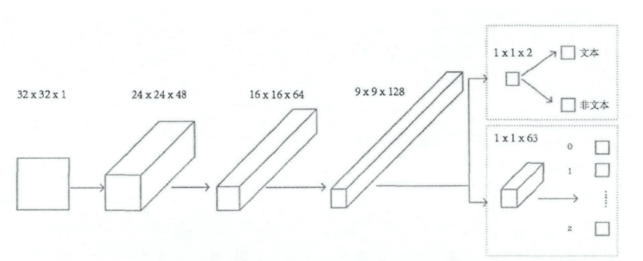
Text recognition in natural scenes - Text recognition classifier Explanation
Preface: In the previous article, we simply explainedText recognition classifier of the convolutional neural network (CNN) classifierIn this article, the text recognition classifier design from the st...
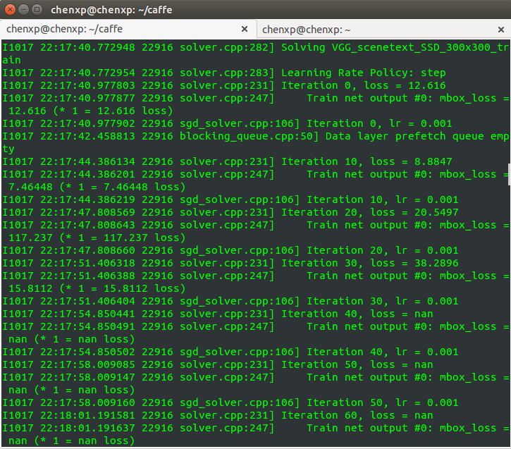
SSD: Signle Shot Detector for text detection in natural scenes
Preface Before i was Paper reading: SSD: Single Shot MultiBox Detector In, talked about the latest Object Detection algorithm. Since SSD is used to detect objects, can SSD be used to detect text in na...

Natural scene text recognition based on deep learning
Statement: The source of this article, please refer to the original blog post for details. 1.1 Introduction Traditional optical character recognition is mainly for high-quality document images....
Survey natural scene text detection and recognition
forward from Green Snake special episode: sister, image text detection and identification of areas of what is now the hot topic? White Snake: black and white scanned document recognition technology ha...
More Recommendation

A Summary of Natural Scene Text Detection and Recognition Technology
Fanwai Green Snake: Sister, what is the current research hotspot in the field of image text detection and recognition? White Snake: The scanning document recognition technology of white and black char...

Overview of natural scene text detection techniques (CTPN, SegLink, EAST)
The article is reproduced from: Foreword Text recognition is divided into two specific steps: the detection of text and the recognition of text, both of which are indispensable, especially text detect...

Python+opencv+EAST to do natural scene text detection (transfer)
Mark, thank the author for sharing! English original link:https://www.pyimagesearch.com/2018/08/20/opencv-text-detection-east-text-detector/ Reminder: Author's implementation of Python's text detectio...
End-to-end text OCR for deep learning: use the EAST model to extract text from natural scene pictures
We live in an era: if any organization or company wants to scale up and remain relevant, it must change their perception of technology and quickly adapt to the changing environment. We already know ho...

Natural scene text detection
Text detection is a prerequisite for text recognition. About the topic Areas of interest, text detection and recognition are full of application requirements in real scenes, and existing algorithms st...