Python confusion matrix visualization [heat map]
tags: python Visualization
Python confusion matrix visualization [heat map]
Dependent package
seaborn with matplotlib Many drawing methods have been provided, and the following methods are all around this
import itertools
import numpy as np
import pandas as pd

import seaborn as sns
import matplotlib.pyplot as plt
Compared
Three implementation methods are given below, and the renderings are as follows:
method 1:
Method 2:
Method 3:

【note】 About each figureColor effects (called color mapping), The color effect of the three methodsCan be changed, See below for details【Color Mapping】 section.
method 1
Code:
def heatmap(data, row_labels, col_labels, ax=None,
cbar_kw={}, cbarlabel="", **kwargs):
"""
Create a heatmap from a numpy array and two lists of labels.
Parameters
----------
data
A 2D numpy array of shape (N, M).
row_labels
A list or array of length N with the labels for the rows.
col_labels
A list or array of length M with the labels for the columns.
ax
A `matplotlib.axes.Axes` instance to which the heatmap is plotted. If
not provided, use current axes or create a new one. Optional.
cbar_kw
A dictionary with arguments to `matplotlib.Figure.colorbar`. Optional.
cbarlabel
The label for the colorbar. Optional.
**kwargs
All other arguments are forwarded to `imshow`.
"""
if not ax:
ax = plt.gca()
# Plot the heatmap
im = ax.imshow(data, **kwargs)
# Create colorbar
cbar = ax.figure.colorbar(im, ax=ax, **cbar_kw)
cbar.ax.set_ylabel(cbarlabel, rotation=-90, va="bottom",
fontsize=15,family='Times New Roman')
# We want to show all ticks...
ax.set_xticks(np.arange(data.shape[1]))
ax.set_yticks(np.arange(data.shape[0]))
# ... and label them with the respective list entries.
ax.set_xticklabels(col_labels,fontsize=12,family='Times New Roman')
ax.set_yticklabels(row_labels,fontsize=12,family='Times New Roman')
# Let the horizontal axes labeling appear on top.
ax.tick_params(top=True, bottom=False,
labeltop=True, labelbottom=False)
# Rotate the tick labels and set their alignment.
plt.setp(ax.get_xticklabels(), rotation=-30, ha="right",
rotation_mode="anchor")
# Turn spines off and create white grid.
for edge, spine in ax.spines.items():
spine.set_visible(False)
ax.set_xticks(np.arange(data.shape[1]+1)-.5, minor=True)
ax.set_yticks(np.arange(data.shape[0]+1)-.5, minor=True)
ax.grid(which="minor", color="w", linestyle='-', linewidth=3)
ax.tick_params(which="minor", bottom=False, left=False)
return im, cbar
def annotate_heatmap(im, data=None, valfmt="{x:.2f}",
textcolors=("black", "white"),
threshold=None, **textkw):
"""
A function to annotate a heatmap.
Parameters
----------
im
The AxesImage to be labeled.
data
Data used to annotate. If None, the image's data is used. Optional.
valfmt
The format of the annotations inside the heatmap. This should either
use the string format method, e.g. "$ {x:.2f}", or be a
`matplotlib.ticker.Formatter`. Optional.
textcolors
A pair of colors. The first is used for values below a threshold,
the second for those above. Optional.
threshold
Value in data units according to which the colors from textcolors are
applied. If None (the default) uses the middle of the colormap as
separation. Optional.
**kwargs
All other arguments are forwarded to each call to `text` used to create
the text labels.
"""
if not isinstance(data, (list, np.ndarray)):
data = im.get_array()
# Normalize the threshold to the images color range.
if threshold is not None:
threshold = im.norm(threshold)
else:
threshold = im.norm(data.max())/2.
# Set default alignment to center, but allow it to be
# overwritten by textkw.
kw = dict(horizontalalignment="center",
verticalalignment="center")
kw.update(textkw)
# Get the formatter in case a string is supplied
if isinstance(valfmt, str):
valfmt = matplotlib.ticker.StrMethodFormatter(valfmt)
# Loop over the data and create a `Text` for each "pixel".
# Change the text's color depending on the data.
texts = []
for i in range(data.shape[0]):
for j in range(data.shape[1]):
kw.update(color=textcolors[int(im.norm(data[i, j]) > threshold)])
text = im.axes.text(j, i, valfmt(data[i, j], None), **kw)
texts.append(text)
return texts
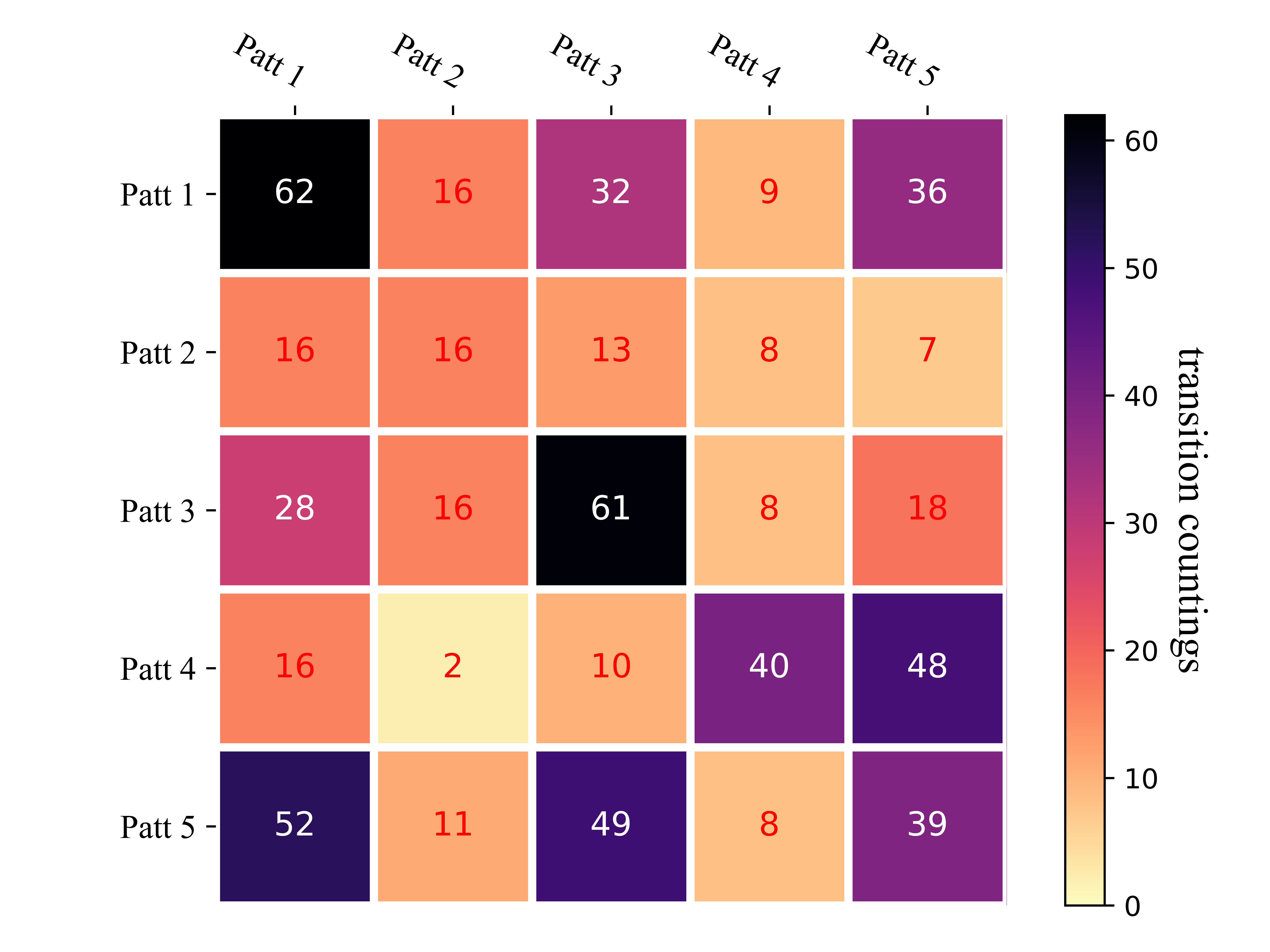
trans_mat = np.array([[62, 16, 32 ,9, 36],
[16, 16, 13, 8, 7],
[28, 16, 61, 8, 18],
[16, 2, 10, 40, 48],
[52, 11, 49, 8, 39]], dtype=int)
"""method 1"""
if True:
np.random.seed(19680801)
ax = plt.plot()
y = ["Patt {}".format(i) for i in range(1, trans_mat.shape[0]+1)]
x = ["Patt {}".format(i) for i in range(1, trans_mat.shape[1]+1)]
im, _ = heatmap(trans_mat, y, x, ax=ax, vmin=0,
cmap="magma_r", cbarlabel="transition countings")
annotate_heatmap(im, valfmt="{x:d}", size=10, threshold=20,
textcolors=("red", "white"), fontsize=12)
# Compact picture effect, easy to save
plt.tight_layout()
plt.savefig('res/method_1.png', transparent=True, dpi=800)
plt.show()
Effect picture:
Method 2
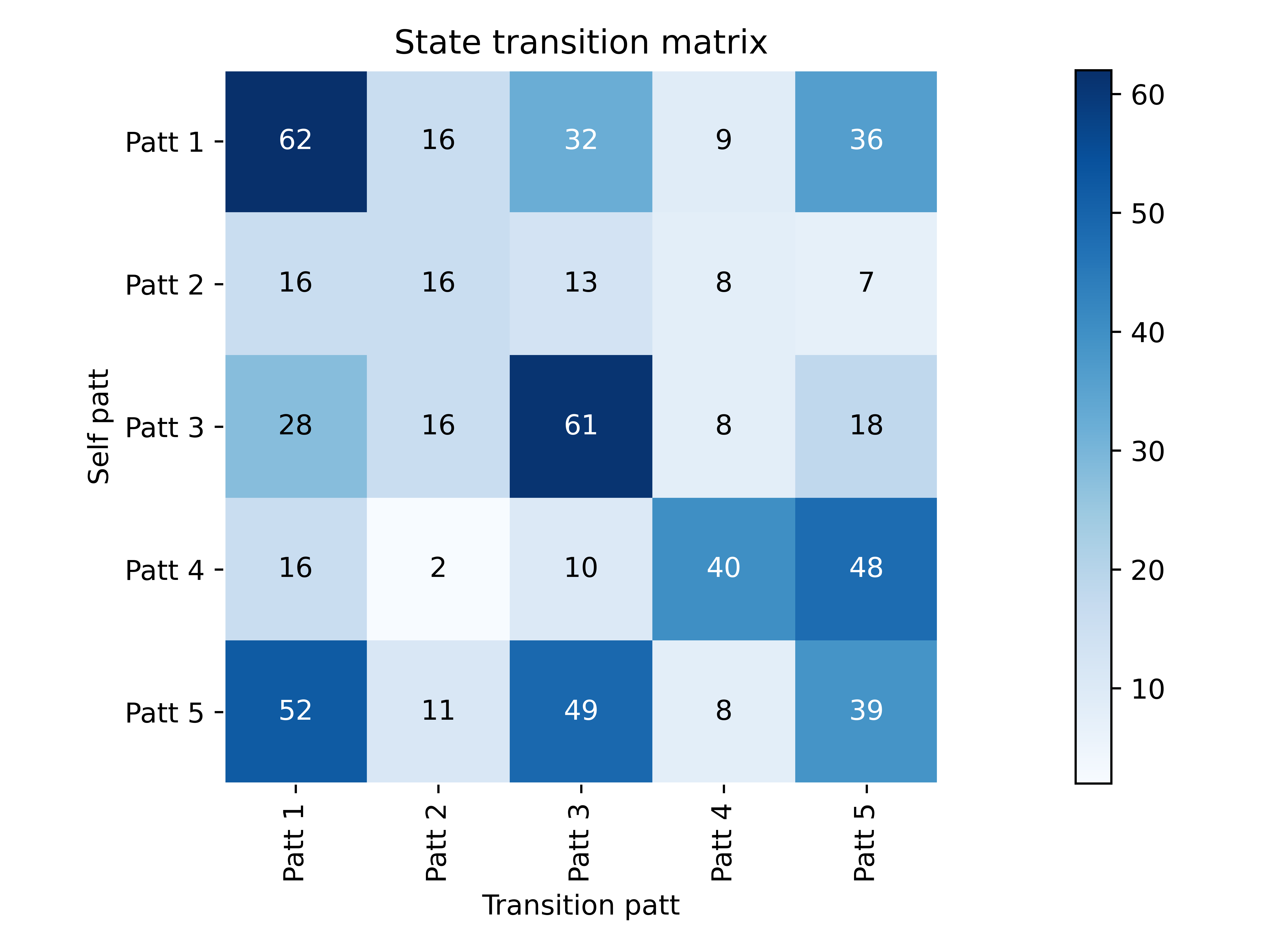
def plot_confusion_matrix(cm, classes, normalize=False, title='State transition matrix', cmap=plt.cm.Blues):

    plt.figure()
    plt.imshow(cm, interpolation='nearest', cmap=cmap)
    plt.title(title)
    plt.colorbar()
    tick_marks = np.arange(len(classes))
    plt.xticks(tick_marks, classes, rotation=90)
    plt.yticks(tick_marks, classes)

    plt.axis("equal")

    ax = plt.gca()
    left, right = plt.xlim()
    ax.spines['left'].set_position(('data', left))
    ax.spines['right'].set_position(('data', right))
    for edge_i in ['top', 'bottom', 'right', 'left']:
        ax.spines[edge_i].set_edgecolor("white")


    thresh = cm.max() / 2.
    for i, j in itertools.product(range(cm.shape[0]), range(cm.shape[1])):
        num = '{:.2f}'.format(cm[i, j]) if normalize else int(cm[i, j])
        plt.text(j, i, num,
                 verticalalignment='center',
                 horizontalalignment="center",
                 color="white" if num > thresh else "black")

    plt.ylabel('Self patt')
    plt.xlabel('Transition patt')

    plt.tight_layout()
    plt.savefig('res/method_2.png', transparent=True, dpi=800)

    plt.show()


trans_mat = np.array([[62, 16, 32 ,9, 36],
                      [16, 16, 13, 8, 7],
                      [28, 16, 61, 8, 18],
                      [16, 2, 10, 40, 48],
                      [52, 11, 49, 8, 39]], dtype=int)

"""method 2"""
if True:
    label = ["Patt {}".format(i) for i in range(1, trans_mat.shape[0]+1)]
    plot_confusion_matrix(trans_mat, label)
Effect picture:
The disadvantage of the above two methods is that they can only accept int type array or dataFrame, and cannot satisfy the state transition matrix drawing with elements less than 1. So consider the third method.
Method 3
trans_mat = np.array([[62, 16, 32 ,9, 36],
[16, 16, 13, 8, 7],
[28, 16, 61, 8, 18],
[16, 2, 10, 40, 48],
[52, 11, 49, 8, 39]], dtype=int)
trans_prob_mat = (trans_mat.T/np.sum(trans_mat, 1)).T
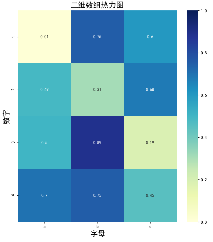
if True:
label = ["Patt {}".format(i) for i in range(1, trans_mat.shape[0]+1)]
df = pd.DataFrame(trans_prob_mat, index=label, columns=label)
# Plot
plt.figure(figsize=(7.5, 6.3))
ax = sns.heatmap(df, xticklabels=df.corr().columns,
yticklabels=df.corr().columns, cmap='magma',
linewidths=6, annot=True)
# Decorations
plt.xticks(fontsize=16,family='Times New Roman')
plt.yticks(fontsize=16,family='Times New Roman')
plt.tight_layout()
plt.savefig('res/method_3.png', transparent=True, dpi=800)
plt.show()
Effect picture:
As you can see, one drawback of this method is that the matrixThe ordinate yticks will be slightly shifted。
【BUG】 Some friends may have the following when using the codeThe first and last lines are not displayed completely The problem.
Solution:
1. Update the matplotlib version. After the actual test is updated to 3.2.0, similar problems no longer occur:
pip install --user --upgrade matplotlib==3.2.0
2. If you don't want to update the version, you can also add the following two lines before plt.show():
bottom, top = ax.get_ylim()
ax.set_ylim(bottom + 0.5, top - 0.5)
discuss
From the perspective of extensibility and universality, the third method may be the best because it isDirect call to seaborn's sns.heatmap() heat map function. Detailed parameter information about the heat map,Official document (http://seaborn.pydata.org/generated/seaborn.heatmap.html) A very comprehensive explanation has been given, so I won't repeat it here.
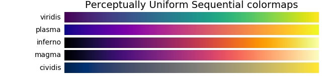
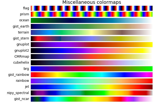
Color mapping
Whether it is plt still is sns, Used in color mappingParameter cmap To represent.
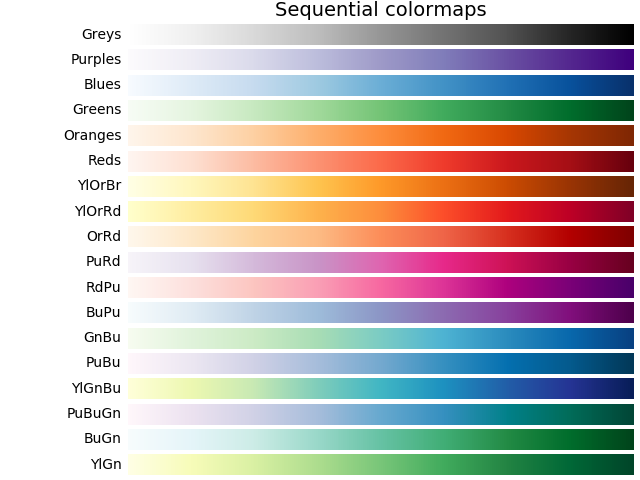
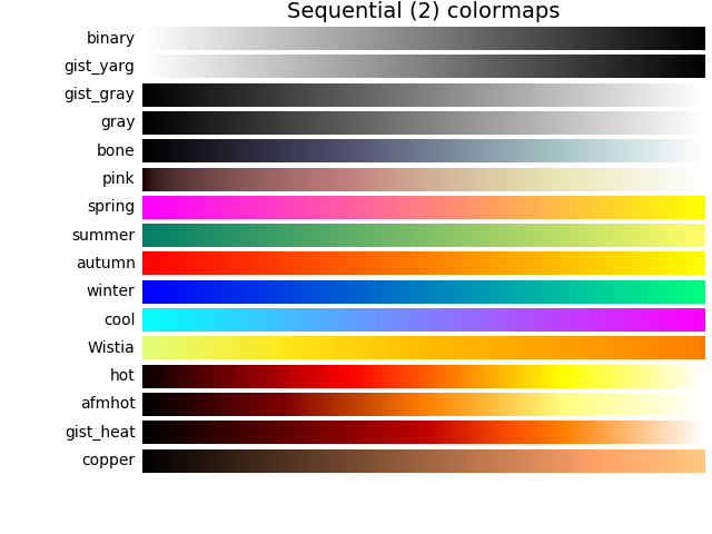
Regarding color mapping, this blog has been written in great detail. For the pursuit of beauty, try more concentrated mapping methods:matplotlib.pyplot.colormaps colormap cmap
-
Sequential:order. Usually usedSingle tone, Gradually change the brightness and the color gradually increases. Should be used to indicateOrdered information。
-
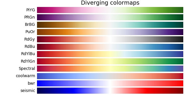
Diverging:Divergence. changeBrightness and saturation of two different colors, These colors meet in an unsaturated color in the middle; this value should be used when the drawn information has a key intermediate value (such as terrain) or the data deviates from zero.
-
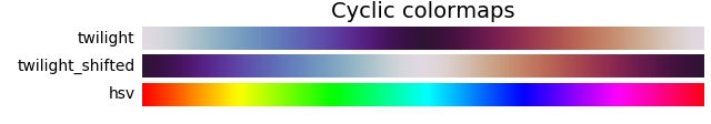
Cyclic: cycle. Change the brightness of two different colors to meet in an unsaturated color in the middle and at the beginning/end. Should be used for values that wrap around the endpoints, such as phase angle, wind direction, or time of day.
-
Qualitative: Qualitative. Often variegated, used to indicate information that has no order or relationship.
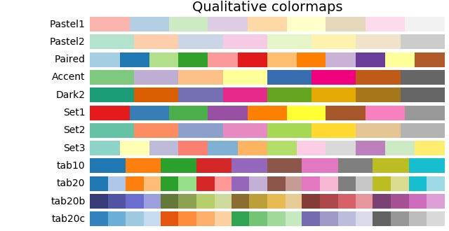
-
Miscellaneous: variegated.
Intelligent Recommendation
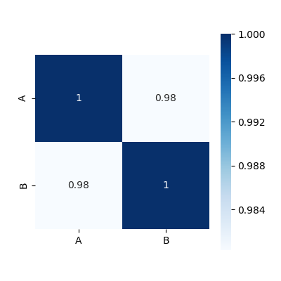
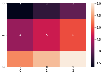
Python correlation coefficient matrix heat map (2)
The above picture is implemented by the following code Simultaneously df The internal data is: A B 0 0.180270 0.019475 1 0.463219 0.724934 2 0.420204 0.485427 Since I set a random number seed, your da...
Confusion matrix and its visualization
Confusion Matrix is used in machine learningSummarize the prediction results of the classification modelAn analysis table of is a commonly used expression in the field of pattern recognition. It dep...

Quant visualization-----Heat map
I was deeply impressed after listening to Nividia's technology on visual computing. If you can present a transaction or data in a graphical way, you can give the most direct feeling. The amount of dat...
More Recommendation

Heat map of data visualization
Reposted from the originalHeat map of data visualization I recently took a look at Baidu'sHeat mapThrough Baidu Maps, it is indeed an image expression form of real-time big data rendering. I just take...
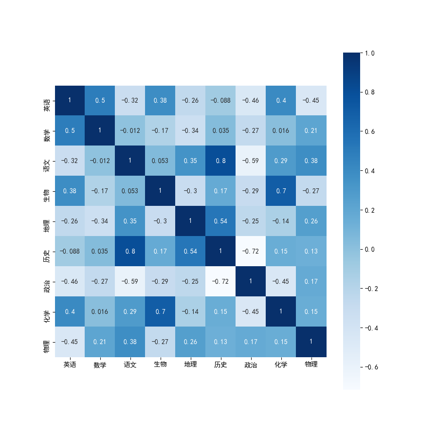
Python draw heat map (correlation coefficient matrix map)
The method of displaying a two-dimensional matrix including a matrix diagram of correlation coefficients in the form of a heat map, currently found two: The first is to use the functions of the pandas...

Python visualization: advanced use of Seaborn library heat map
Foreword In daily work, you can often see all kinds of exquisite heat maps. The heat maps are widely used. Let's learn how to use heat maps in Python's Seaborn library. The environment for this run is...

Python visualization advanced --- seaborn1.9 timeline chart, heat map tsplot () / heatmap ()
Timeline charts, heat maps tsplot() / heatmap() 1. Timeline chart-tsplot () Example 1: Example 2: Example 3: 2. Heatmap-heatmap () Example 1: Example 2: Setting parameters Example 3: Drawing a half-ed...
Python is based on PyeCharts custom latitude and longitude heat map visualization
background In the analysis of business data statistical analysis, the analysis of the provinces and regions will be basically involved. Data visualization is a tool for data analysis. The data of thes...