How to implement the FFT analysis of PowerGUI in Simulink?
Disclaimer: The author has not successfully achieved it, and has not even obtained a normal FFT analysis result.
Matlab version: 2020B
Simulink Seeking solution: Auto (ODE3TB), running long running
The first is how to use PowerGUI in Simulink for FFT analysis.
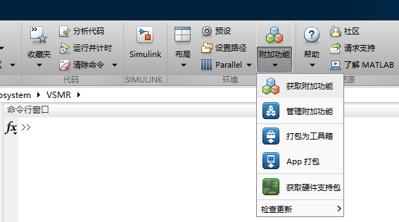
PowerGUI's path in Simulink Library Browser is SimsCape/Electrical/Specialized Power System/Fundammental Blocks. Drag the PowerGui into Simulink to complete the layout.
FFT has been marked with a red box in the figure.
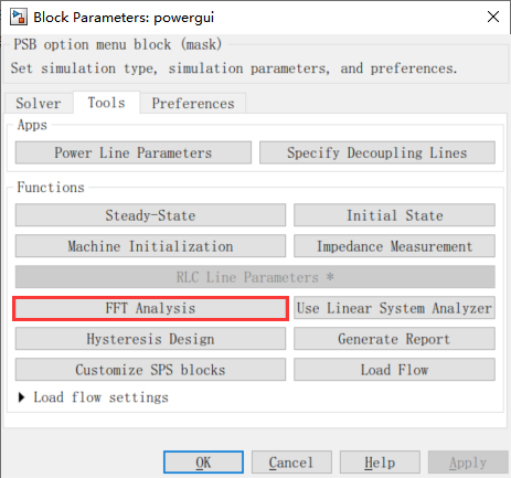
In order to use FFT Analysis, some other settings are needed.
a. Get the signal
The signal in FFT comes from Scope and needs to be set on scope. The red box is a key setting. The variable name is casual. The data will be stored in the work area at the same time, and it is also convenient for secondary analysis in the work area.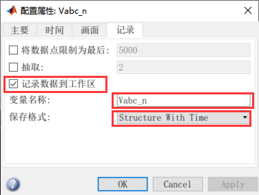
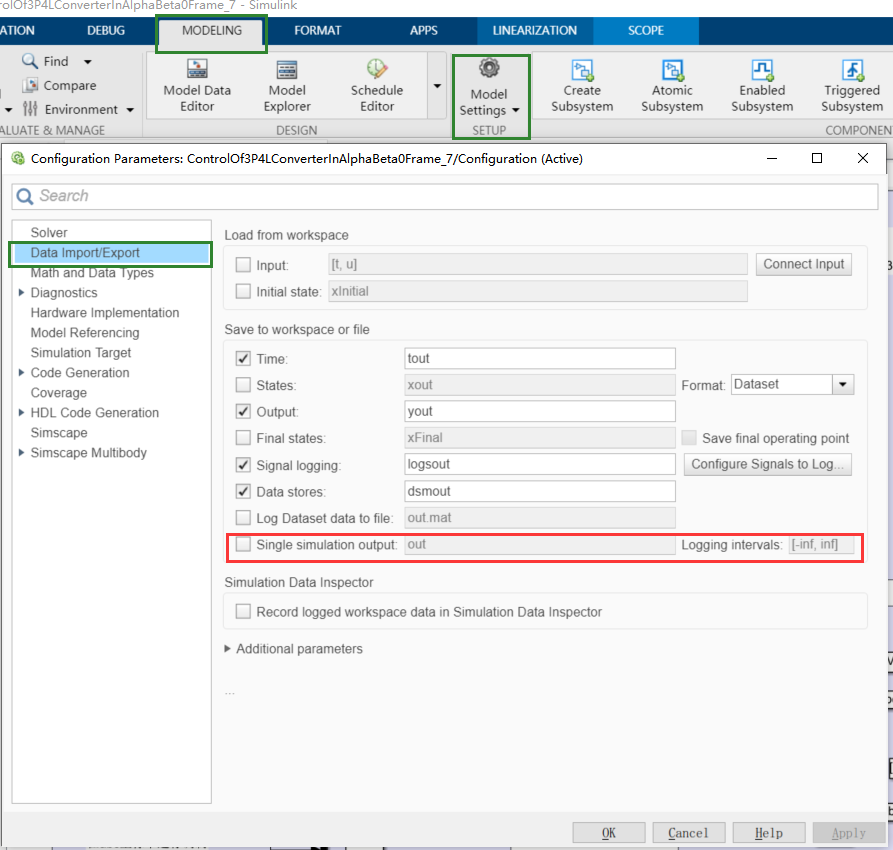
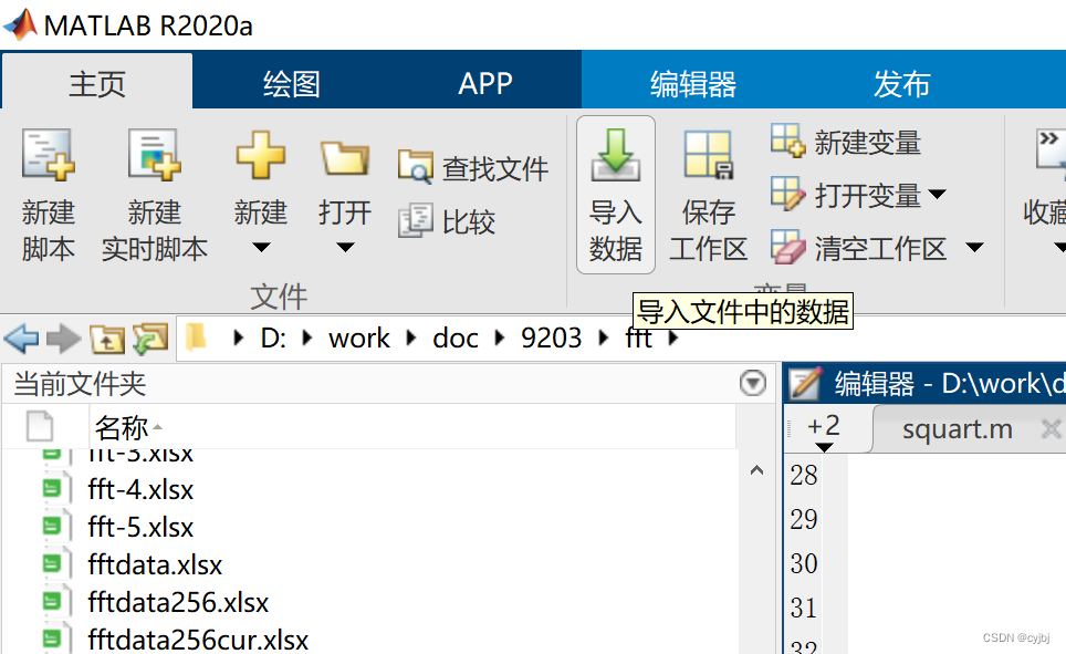
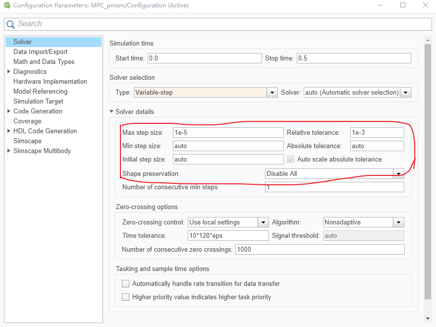
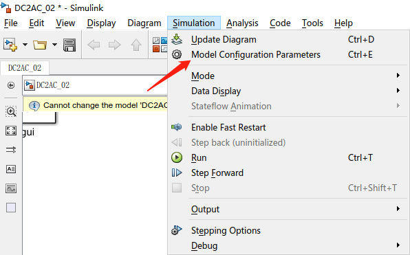
2. Model parameters
The green frame in the figure gives the setting path. Don't choose in the red box.
After setting, reorganize the simulation to get data and enter FFT analysis. Proceed as follows.
Use PowerGUI for FFT analysis, simple and easy to get started, and the results are intuitive. And you can see THD.
But it is not convenient to obtain some characteristic frequency content. So think of using the M file to implement FFT analysis.
Note that after the above settings, the Simulink file will generate a structure variable in the work area after running.
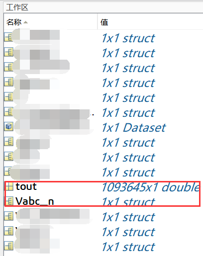
The data in VABC_N is as follows:
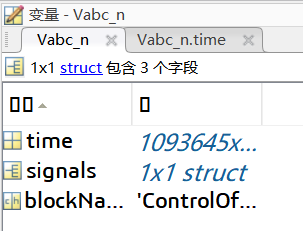
Vabc_n.time is stored in each sampling point. Signal data is stored in VABC_N.Signals.
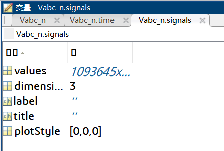
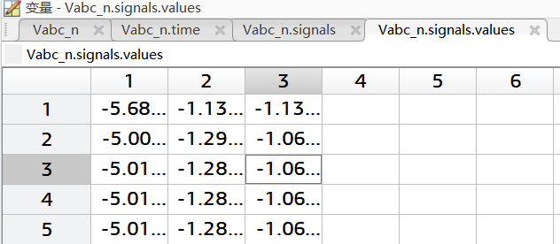
The sampling data in VABC_N.Signals.Values.
Then FFT analysis can be performed on the structure variable.
Since the author has never used the FFT function. View the routine with DOC FFT.
The code about Yu Xianbo is as follows:
English annotation is an annotation that comes with the routine, and the Chinese annotation is added to the author.
Fs = 1000; % Sampling frequency
T = 1/Fs; % Sampling period
L = 1000; % Length of signal
t = (0:L-1)*T; % Time vector
x1 = cos(2*pi*50*t); % First row wave
x2 = cos(2*pi*150*t); % Second row wave
x3 = cos(2*pi*300*t); % Third row wave
X = [x1; x2; x3];
n = 2^nextpow2(L); %In order to optimize the FFT performance, the signal length needs to be guaranteed2The power second.
dim = 2; %FFT is performed on each line of the signal. By default1That is to perform FFT analysis of each column.
Y = fft(X,n,dim);
P2 = abs(Y/L); %Bilateral spectrum
P1 = P2(:,1:n/2+1); %Unilateral spectrum
P1(:,2:end-1) = 2*P1(:,2:end-1);
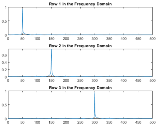
for i=1:3 %Display spectrum analysis results
subplot(3,1,i)
plot(0:(Fs/n):(Fs/2-Fs/n),P1(i,1:n/2))
title(['Row ',num2str(i),' in the Frequency Domain'])
end
The running results are as follows:
According to this, the author wrote the following code
function output = FFTofSignal(signals)
if class(signals)=="struct"
    L = length(signals.time);
%     In order to consider algorithm performance, the signal length is best2Power secondary value
    n = 2^nextpow2(L);
%          Obviously, n/2<L<n, the length of the signal can be n/2Or N/4hour,3LMay be exceeded, so take n/8。
    L = n/8;
    t = signals.time(L:3*L);    %Analyze the middle section of the signal, this is the intercept time
    Fs = (length(t)-1)/(t(end)-t(1));   %Sampling frequency=Data point number/length of time
    X = signals.signals.values(L:3*L,:);    %Intercept the signal
    Y = fft(X,L,1);                     %FFT analysis
    P2 = abs(Y/L);                      %Calculate bilateral spectrum
    P1 = P2(1:L/2+1,:);                   %Unilateral spectrum
    P1(2:end-1,:) = 2*P1(2:end-1,:);
    f = Fs*(0:(L/2))/L;
    output = figure;
    subplot(2,1,1)
    plot(t,X);                      %Output signal
    subplot(2,1,2)
    plot(f,P1);                     %Output FFT analysis results
    title('Single-Sided Amplitude Spectrum of X(t)')
    xlabel('f (Hz)')
    ylabel('|P1(f)|')
else
    output = [];
    disp("The signal type is the structure, please confirm before entering")
end
Run Temp = fftofsignal (vabc_n); get the figure below. The results of the original data chart and FFT analysis have magnified the area.
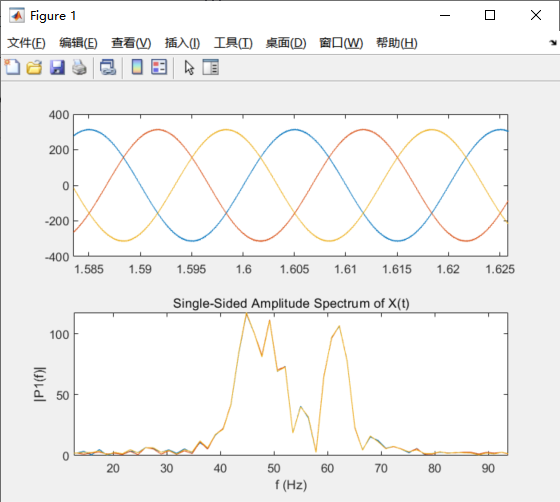
You can see that the analysis results are not good. In the original data, the harmonic content is small, and it can be approximately considered to contain a base wave component of only 50Hz. The FFT analysis results present a large number of other frequencies.
But I don't know why.
In response to this issue, do you have any suggestions?
Intelligent Recommendation
Use matlab programming to implement FFT spectral analysis
Table of contents Use matlab programming to implement FFT spectral analysis FFT function Original waveform function Original data import function Data export function FFT analysis routine Use matlab p...
The relationship between Simulink medium step size, powergui sampling time, module sampling time, control period
The relationship between Simulink medium step size, powergui sampling time, module sampling time, control period Recently, when I was building a model, I had conceptual confusion about the various &qu...
[Simulink Module] S-Function S Function Module - How to Implement the Real Time Change in the Simulink Simulation
In the process of using Simulink, you will often encounter a problem. I hope that I have changed in the module (a MASK) in the module. For example, 1. I want to simulate a sudden change in load resist...
MATLAB | How to implement Simulink simulation time is equal to real time
table of Contents 1 Overview 2. Install the plugin 3. Use the plugin 1 Overview Previous article "MATLAB | Simulink simulation time with actual time synchronization settings"Describes the fu...

How does MATLAB implement the Fourier transform FFT? What is the physical meaning?
How does MATLAB implement the Fourier transform FFT? What is the physical meaning? Step by step Why do you want to make a Fourier transform, what is the point? How to implement fast Fourier transform ...
More Recommendation
☆Power Electronic Technology☆Use of FFT Tools in simulink
Use of FFT Tools in simulink 1. Build a simulation circuit 2. Set the simulation to a discrete environment 3. Configure powergui 4. Connect the oscilloscope and powergui 5. Run the program 6. Open the...
Analysis of Fixed-step size (in Solver), Sample time (in module), and Sample time (in powergui)
Analysis of Fixed-step size (in Solver), Sample time (in module), and Sample time (in powergui) Because no official explanation can be found to clearly explain the relationship between the three, this...
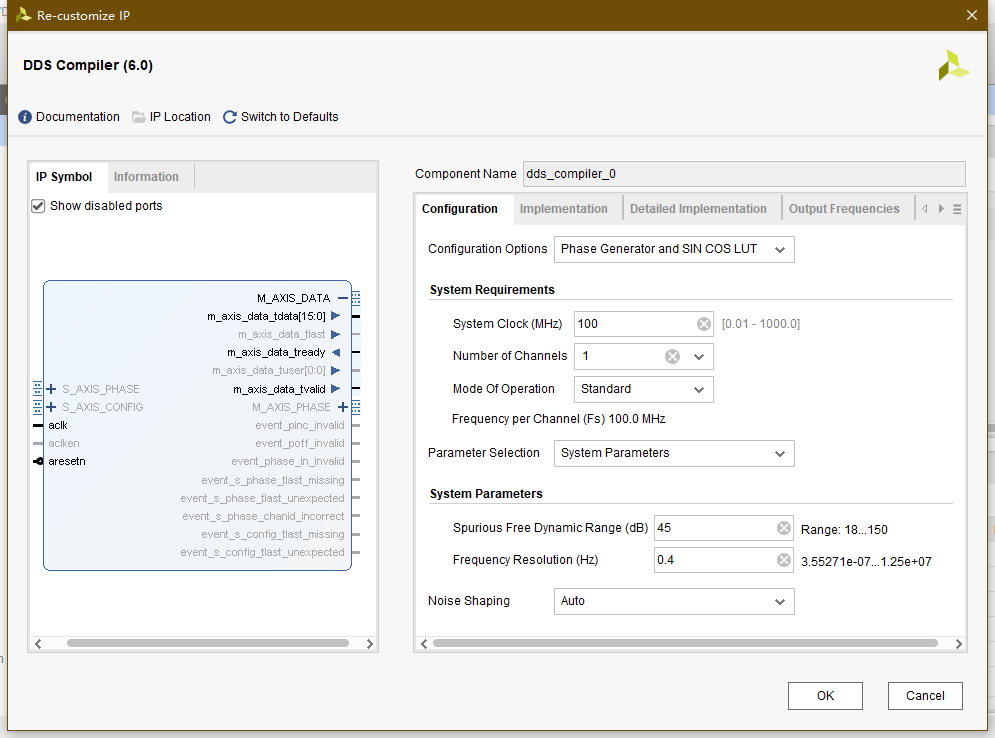
Implement FFT/IFFT in VIVADO
The main idea: (this should be the easiest way) DDS generates a fixed frequency quadrature signal Instantiate two FFTIP cores respectively as FFT cores for IFFT transformation Input the DDS signal to ...
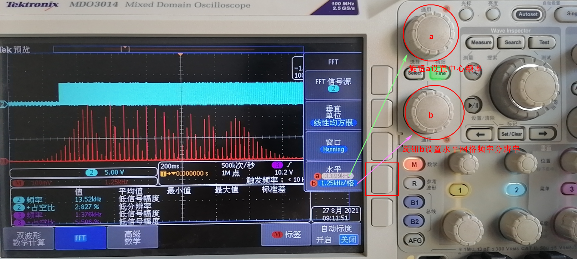
How to use the FFT function of waveform frequency analysis of Tektronix oscilloscope MDO3014
Generally, when viewing a waveform with an oscilloscope, the frequency parameters of the waveform are directly displayed. If the frequency of the waveform does not change much, it is more conven...

Simulink analysis of Daphne equation
See the Wikipedia for the Duffing equation: https://en.wikipedia.org/wiki/Duffing_equation Use the simulink to build the Duffin equation model as shown below: When the stiffness coefficient is 0, the ...