LASSO Proximal Gradient Descent formula derivation and code
tags: Machine learning Python optimization
Article Directory
LASSO by Proximal Gradient Descent
Prepare:
from itertools import cycle
import numpy as np
import matplotlib.pyplot as plt
from sklearn.linear_model import lasso_path, enet_path
from sklearn import datasets
from copy import deepcopy

X = np.random.randn(100,10)
y = np.dot(X,[1,2,3,4,5,6,7,8,9,10])
Proximal Gradient Descent Framework
- randomly set for iteration 0
- For
th iteration:
----Compute gradient
----Set
----Update
----Check convergence: if yes, end algorithm; else continue update
Endfor
Here
, and
,
where the size of
,
,
is
,
,
, which means
samples and
features. Parameter
can be chosen, and
can be considered as step size.
Proximal Gradient Descent Details
Consider optimization problem:
where
,
. And
is differentiable convex function, and
is convex but may not differentiable.
For
, according to Lipschitz continuity, for
, there always exists a constant
s.t.
Then this problem can be solved using Proximal Gradient Descent.
Denote
as the
th updated result for
, then for
, the proximation of
can be a function of
and
:
where
is not related with
, so can be ignored.
The original solution for
at iteration
is
In proximal gradient method, we use below instead:
Given
, and let
, we have
To solve Equation above, let
. For
th element in
, it’s easy to know that the optimal
satisfies
and we can get
.
The goal is to express
as a function of
.This can be done by swapping the
-
axes of the plot of
:
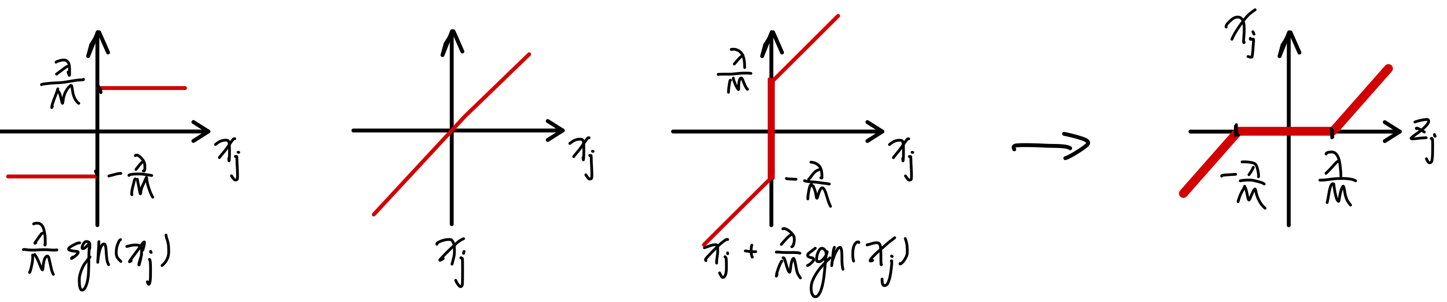
Then
can be expressed as
Simplified Code
The code is Python version of proximal gradient descent from Stanford MATLAB LASSO demo.
In the original code, to make sure the differentiable part of objective function
will decrease after each time weight update, there is a check to see whether the first-order approximation of
is smaller than the value from previous
:
def f(X, y, w):
    n_samples, _ = X.shape
    tmp = y - np.dot(X,w)
    return 2*np.dot(tmp, tmp) / n_samples

def objective(X,y,w,lmbd):
    n_samples, _ = X.shape
    tmp = y - np.dot(X,w)
    obj_v = 2 * np.dot(tmp,tmp) / n_samples + lmbd * np.sum(np.abs(w))
    return obj_v


def LASSO_proximal_gradient(X, y, lmbd, L=1, max_iter=1000, tol=1e-4):
    beta = 0.5 # used to update L for finding proper step size
    n_samples, n_features = X.shape
    w = np.empty(n_features, dtype=float)
    w_prev = np.empty(n_features, dtype=float) # store the old weights
    xty_N = np.dot(X.T, y) / n_samples
    xtx_N = np.dot(X.T, X) / n_samples
    prox_thres = lmbd / L
    h_prox_optval = np.empty(max_iter, dtype=float)
    for k in range(max_iter):
        while True:
            grad_w = np.dot(xtx_N, w)- xty_N
            z = w - grad_w/L
            w_tmp = np.sign(z) * np.maximum(np.abs(z)-prox_thres, 0)
            w_diff = w_tmp - w
            if f(X, y, w_tmp) <= f(X, y, w) + np.dot(grad_w, w_diff) + L/2 * np.sum(w_diff**2):
                break
            L = L / beta
        w_prev = copy(w)
        w = copy(w_tmp)

        h_prox_optval[k] = objective(X,y,w,lmbd)
        if k > 0 and abs(h_prox_optval[k] - h_prox_optval[k-1]) < tol:
            break
    return w, h_prox_optval[:k]

def pgd_lasso_path(X, y, lmbds):
    n_samples, n_features = X.shape
    pgd_coefs = np.empty((n_features, len(lmbds)), dtype=float)
    for i, lmbd in enumerate(lmbds):
        w, _ = LASSO_proximal_gradient(X, y, lmbd)
        pgd_coefs[:,i] = w
    return lmbds, pgd_coefs
experiment:
lmbds, pgd_coefs = pgd_lasso_path(X, y, my_lambdas)
# Display results
plt.figure(1)
colors = cycle(['b', 'r', 'g', 'c', 'k', 'y','m'])
neg_log_lambdas_lasso = -np.log10(my_lambdas)
for coef_l, c in zip(coefs_lasso, colors):
    l1 = plt.plot(neg_log_lambdas_lasso, coef_l, c=c)

plt.xlabel('-Log($\lambda$)')
plt.ylabel('coefficients')
plt.title('PGD Lasso Paths')
plt.axis('tight')
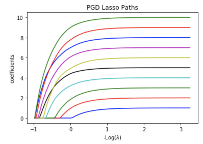
the result looks similar with that using Coordinate Descent Method
Speed Comparison
print("Coordinate descent method from scikit-learn:")
%timeit lambdas_lasso, coefs_lasso, _ = lasso_path(X, y, eps, fit_intercept=False)

print("PGD method:")
%timeit lmbds, pgd_coefs = pgd_lasso_path(X, y, my_lambdas)
Results:
Coordinate descent method from scikit-learn:
4.88 ms ± 97 µs per loop (mean ± std. dev. of 7 runs, 100 loops each)

PGD method:
778 ms ± 21.3 ms per loop (mean ± std. dev. of 7 runs, 1 loop each)
Pure python PGD is faster than that of coordinate descent method in my previous blog, but slower than Cython coordinate descent method.
Intelligent Recommendation

Logistic (log probability) regression through gradient descent, including formula derivation and code implementation
As we all know, the logistic regression algorithm is a very classic machine learning algorithm that can be used for regression and classification tasks. It is also a linear regression model in a broad...

Mathematical Derivation of Gradient Descent Formula of Logistic Regression Cost Function
The Derivation Process of Gradient Descent Formula of Logistic Regression Cost Function Logistic regression cost function gradient descent formula mathematical derivation process The mathematical deri...

Derivation process of gradient descent formula (Wu Enda course)
The course is when the gradient is falling. There is a formula. As shown below The difficulty is the derivation process. The results are as follows: But the teacher gave the answer directly. Did not e...

Logtic regression loss function and gradient descent formula derivation
Logistic regression cost function derivation process. The algorithm solution uses the following cost function form: Gradient descent algorithm For a function, we need to find its minimum...
The gradient descent algorithm and its promotion algorithm involve formula derivation
Gradient descent algorithm ideas and other popularization algorithms This article introduces the general format of gradient descent, Gradient descent algorithm (small batch, batch, random), Formula de...
More Recommendation

Gradient Descent Derivation and Examples
Gradient Descent Derivation and Examples Note: The author organizes on the basis of other literatures to form the basic context of this article, and hopes to help beginners through a simpler and clear...
Gradient descent method derivation
** Gradient descent method formula derivation ** The gradient descent method is simply a method of finding the minimum point. It is a commonly used optimizer in machine learning and deep learning. Spe...
Derivation of gradient descent
Derivation of gradient descent 01. Problem 02. What is gradient 03. Gradient derivation 3.1 First-order Taylor Expanded 3.2 Inference on gradient descent method 04. What is gradient descent used for? ...
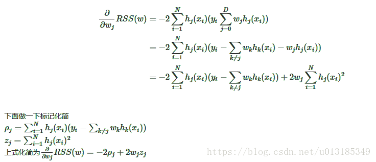
Lasso regression method of coordinate descent derivation
Lasso regression method of coordinate descent derivation The objective function Lasso L1 corresponds with positive linear regression of the term. Look under the objective function: This problem is a r...

Derivation of Lasso regression's coordinate descent method
Objective function Lasso is equivalent to linear regression with L1 regularization term. First look at the objective function: RSS(w)+λ∥w∥1=∑Ni=0(yi−∑Dj=0wjhj(xi))2+λ∑D...