pytorch implements BiLSTM+CRF

​Many tutorials on the Internet are based on the interpretation of the pytorch official website example, so I decided to read the official website example and then reproduce it myself. This article is my detailed interpretation of the official code.

Understanding LSTM

Reference: http://colah.github.io/posts/2015-08-Understanding-LSTMs/

This English LSTM article is really well written. After reading it, I easily picked up the forgotten knowledge.

​ RNN

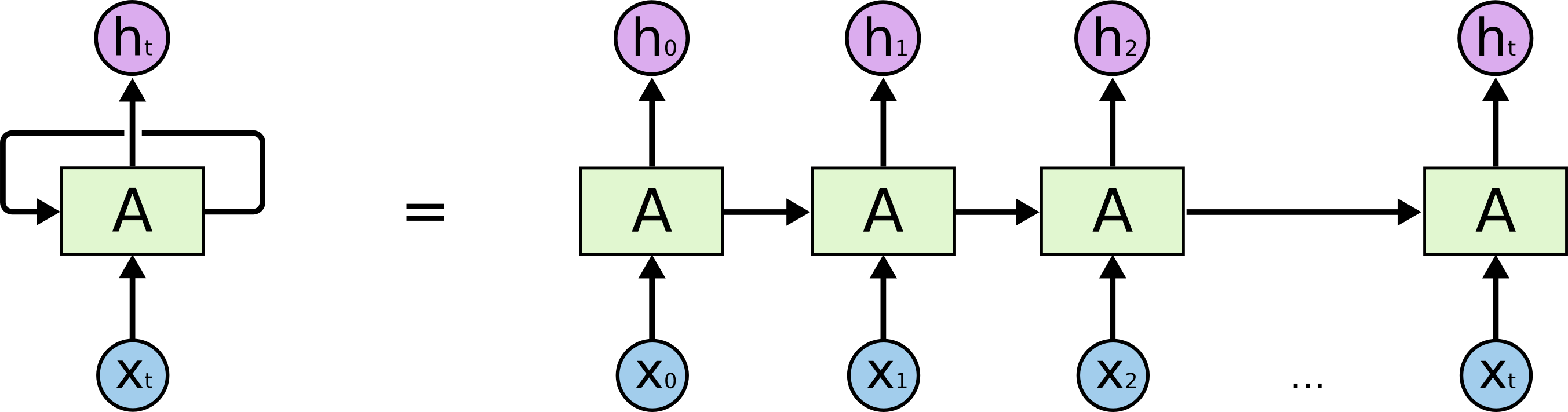
​Although RNN can help us contact the previous information, but when the distance between the relevant information is large, RNN can not work so effectively, then LSTM is needed, the structure of LSTM is shown in the following figure:

[External chain image transfer failed, the source site may have an anti-theft chain mechanism, it is recommended to save the image and upload it directly (img-WFVGTFNr-1579522756021) (http://colah.github.io/posts/2015-08-Understanding-LSTMs /img/LSTM3-chain.png)]

​ The repeating module in an LSTM contains four interacting layers.

The core of LSTM

​The key to LSTM is the state of the unit, a bit like a conveyor belt. It extends along the entire chain along a straight line, with only a few small linear interactions, so information flows very easily without change. The LSTM gate is only based on this straight line. Do some control.

Step by step interpretation of LSTM

​The first step of LSTM is the forget gate, which determines what information we lose in this step. The value of the forget gate is 1 for complete retention, and the value 0 for complete forget.

The second step of LSTM is to determine what new information to store in the unit state, including two parts. First, the input layer uses sigmoid calculation to determine which values ​​will be updated; next, the tanh layer creates a new candidate value $\tilde C_t$C~t​Vector.

​The next step is to update the unit status. You can easily list the expressions according to the illustration.

​The last thing is to determine the output of LSTM. First, we use a sigmoid function to determine which part of the output unit state, and then pass the unit state through the tanh layer and multiply it with the sigmoid value so that we only output the part we want.

Understanding BiLSTM and CRF

Reference: https://www.jianshu.com/p/97cb3b6db573

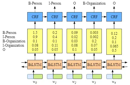
​The output of the BiLSTM layer is the predicted score of each label, and then the output value of BiLSTM is used as the input of the CRF layer. The final result is the label of each word.

The role of the CRF layer

​Although BiLSTM can complete the labeling work, there is no way to add constraints, and constraints can be added through the CRF layer to make the predicted labels legal.

Understand the loss function

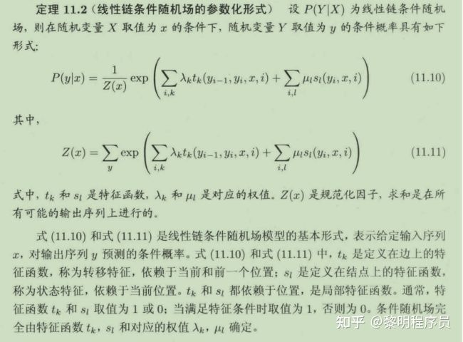
​Assume that our tags have a total of tag_size, then the output dimension of BiLSTM is tag_size, which means each word $w_i$wi​The emission probability value (feats) mapped to the tag, let the output matrix of BiLSTM be $P$P,among them $P_{i,j}$Pi,j​Representative word $w_i$wi​Map to $tag_j $Non-normalized probability. For CRF, we assume that there is a transition matrix$ofnon-ReturnOneChangeGeneralrate。CorrectinCRFComeSay，IWefalsesetSaveinOneAturnshiftMomentFormationA $,then$，thenA_{i,j} $representative$generationtabletag_i $move to$turnshiftToThe transfer probability of tag_j$.

For input sequence $X$XCorresponding output $tag$tagsequence $y$y, Define the score as:
$s(X,y)=\sum_{i=0}^nA_{y_i,y_{i+1}}+\sum_{i=1}^nP_{i,y_i}$s(X,y)=i=0∑n​Ayi​,yi+1​​+i=1∑n​Pi,yi​​
​The softmax processing of the above formula, we all know that softmax can help us map some inputs to real numbers between 0-1, and can be normalized to ensure that the sum is 1, so for The sum of the probability of a word to each tag is 1. Now we use the softmax function for each correct $tag$tagsequence $y$yDefine a probability value ( $Y_X$YX​On behalf of all $tag$tagSequence, including impossible
$p(y|X)=\frac{e^{s(X,y)}}{\sum_{\tilde y\in Y_X}e^{s(X,\tilde y)}}$p(y∣X)=∑y~​∈YX​​es(X,y~​)es(X,y)​
Use logarithmic maximum likelihood estimation
$\log(p(y|X))=S(X,y)-log(\sum_{\tilde y\in Y_X}e^{s(X,\tilde y)})$log(p(y∣X))=S(X,y)−log(y~​∈YX​∑​es(X,y~​))
So Loss can be:
$Loss=\log(\sum_{\tilde y\in Y_X}e^{S(X,\tilde y)})-S(X,y)$Loss=log(y~​∈YX​∑​eS(X,y~​))−S(X,y)

among them $\log(\sum_{\tilde y\in Y_X}e^{S(X,\tilde y)})$log(∑y~​∈YX​​eS(X,y~​))The calculation of is more complicated, because you need to calculate the score of each possible path, you can use a simple method, for the word $w_{i+1}$wi+1​The path to $w_i$wi​The value of is calculated because:
$\log(\sum e^{\log(\sum e^x)+y})=\log(\sum\sum e^{x+y})$log(∑elog(∑ex)+y)=log(∑∑ex+y)

Interpret the code

​ First, let's take a look at the overall idea of ​​the code. Let's start with the training of the model without looking at the implementation of the model.

Training model

​The BIO label is used here, but two more labels are added<START>with<STOP>So our total number of labels is 5

​BIO annotation: B means the beginning of the entity name, I means the middle word of the entity name, O means the non-entity word

'''Functions needed during training'''
def prepare_sequence(seq, to_ix):
    #seq is the corpus after word segmentation, to_ix is ​​the number corresponding to each word in the corpus
    idxs = [to_ix[w] for w in seq]
    return torch.tensor(idxs, dtype=torch.long)

START_TAG = "<START>"
STOP_TAG = "<STOP>"
EMBEDDING_DIM = 5 # Since there are 5 B\I\O\START\STOP tags in total, embedding_dim is 5
HIDDEN_DIM = 4 # This is actually the number of features of the hidden layer of BiLSTM, because it is bidirectional, it is twice, unidirectional is 2

# Training data
training_data = [(
    "the wall street journal reported today that apple corporation made money".split(), #['the','wall','street','journal',...]
    "B I I I O O O B I O O".split() #['B','I','I',...]
), (
    "georgia tech is a university in georgia".split(),
    "B I O O O O B".split()
)]

# Encode each word that is not repeated, for example, ‘HELLO WORLD’ is {'HELLO':0,'WORLD:1'}
word_to_ix = {} # Training dictionary of the corpus, the code corresponding to each word in the corpus (index)
for sentence, tags in training_data:
    for word in sentence:
        if word not in word_to_ix:
            word_to_ix[word] = len(word_to_ix)

tag_to_ix = {"B": 0, "I": 1, "O": 2, START_TAG: 3, STOP_TAG: 4}# Tag dictionary, each tag corresponds to an encoding

model = BiLSTM_CRF(len(word_to_ix), tag_to_ix, EMBEDDING_DIM, HIDDEN_DIM) #model
optimizer = optim.SGD(model.parameters(), lr=0.01, weight_decay=1e-4) #Optimizer, using stochastic gradient descent

# Check predictions before training
with torch.no_grad():
    precheck_sent = prepare_sequence(training_data[0][0], word_to_ix)
    precheck_tags = torch.tensor([tag_to_ix[t] for t in training_data[0][1]], dtype=torch.long)
    print(model(precheck_sent)) #(tensor(2.6907), [1, 2, 2, 2, 2, 2, 2, 2, 2, 2, 1])

# Make sure prepare_sequence from earlier in the LSTM section is loaded
for epoch in range(300): #Cycle times can be set by yourself
    for sentence, tags in training_data:
        # Step 1. Remember that Pytorch accumulates gradients.
        # We need to clear them out before each instance
        model.zero_grad()

        # Step 2. Get our inputs ready for the network, that is,
        # turn them into Tensors of word indices.
        sentence_in = prepare_sequence(sentence, word_to_ix)
        targets = torch.tensor([tag_to_ix[t] for t in tags], dtype=torch.long)

        # Step 3. Run our forward pass.
        loss = model.neg_log_likelihood(sentence_in, targets)

        # Step 4. Compute the loss, gradients, and update the parameters by
        # calling optimizer.step()
        loss.backward()
        optimizer.step()

# Check predictions after training
with torch.no_grad():
    precheck_sent = prepare_sequence(training_data[0][0], word_to_ix)
    print(model(precheck_sent))
# We got it!

Create a model

Interpret the functions in the model step by step, first is initialization

def __init__(self, vocab_size, tag_to_ix, embedding_dim, hidden_dim):
    '''
             Initialize the model
      parameters：
      		       vocab_size: the length of the dictionary of the corpus
      		       tag_to_ix: dictionary of tags and corresponding numbers
      		       embedding_dim: the number of tags
      		hidden_dim: the number of neurons in the hidden layer of BiLSTM
      '''
    super(BiLSTM_CRF, self).__init__()
    self.embedding_dim = embedding_dim
    self.hidden_dim = hidden_dim
    self.vocab_size = vocab_size
    self.tag_to_ix = tag_to_ix
    self.tagset_size = len(tag_to_ix)
    #Output as a mini-batch*words num*embedding_dim matrix
    #vocab_size indicates how many words there are, and embedding_dim indicates how many dimensional vectors you want to create for each word
    self.word_embeds = nn.Embedding(vocab_size, embedding_dim)
    #Create LSTM (the number of features of each word, the number of features of hidden layers, the number of circular layers refers to the number of stacked layers, whether it is BLSTM)
          self.lstm = nn.LSTM(embedding_dim,hidden_dim//2,num_layers=1,bidirectional=True)

    # Map the output of LSTM to the label space
    self.hidden2tag = nn.Linear(hidden_dim, self.tagset_size)

    # Transition matrix, transitions[i][j] represents the probability of transition from label j to label i, although it is randomly generated, it will be updated iteratively later
    # Special note here is that transitions[i] indicates the probability of other tags going to tag i
    self.transitions = nn.Parameter(torch.randn(self.tagset_size,self.tagset_size))

    # These two statements enforce such constraints: we will never transfer to the start tag, and will never transfer from the stop tag
    self.transitions.data[tag_to_ix[START_TAG], :] = -10000#Transfer from any tag to START_TAG impossible
    self.transitions.data[:, tag_to_ix[STOP_TAG]] = -10000#Transfer from STOP_TAG to any tag is impossible

    self.hidden = self.init_hidden()
                         
def init_hidden(self):
    #（num_layers*num_directions,minibatch_size,hidden_dim）
    # Actually initialized h0 and c0
    return (torch.randn(2, 1, self.hidden_dim // 2),
    
            torch.randn(2, 1, self.hidden_dim // 2))

Explain a few important functions in it, it will be of great help to understand the program.

nn.Embedding()

Reference: https://blog.csdn.net/david0611/article/details/81090371

​The function of this function is to create a word embedding model in the form ofnn.Embedding(vocab_size,embedding_dim), Vocab_size indicates how many words there are in the provided corpus, and embedding_dim indicates that you want to create a vector of how many dimensions each word creates (generally the number of tags). The generated model can read multiple vectors, the input is two dimensions (the size of the batch, the number of words in each batch), and the output is the size of the word vector in two dimensions.

embedding = nn.Embedding(10, 3)
# Take two groups per batch, each group of four words, each word is represented by a 3-dimensional vector
input = Variable(torch.LongTensor([[1,2,4,5],[4,3,2,9]]))
a = embedding(input) # Output 2*4*3

nn.LSTM()

Reference: https://blog.csdn.net/rogerfang/article/details/84500754

LSTM() has a total of 7 parameters, only the parameters used here are introduced, input_size refers to the dimension of the input feature (here refers to the dimension of each word after encoding is the number of tags), hidden_size refers to the dimension of the hidden state, num_layers refers to the number of layers in the LSTM stack, that is, whether multiple LSTMs need to be repeated, and setting bidirectional to True means that a bidirectional LSTM is created.

After the model is created, the input and output are shown below:

nn.LSTM(	(Input_size	Hidden_size	Num_layers)
x	Seq_len	batch	Input_size
h0	Num_layers*num_directions	batch	Hidden_size
c0	Num_layers*num_directions	batch	Hidden_size
output	Seq_len	batch	Num_directions*hidden_size
hn	Num_layers*num_directions	batch	Hidden_size
cn	Num_layers*num_directions	batch	Hidden_size

After the model is created, let's take a look at what we do during the process

def forward(self, sentence):  #sentence is an encoded sentence
    # Get the emission scores from the BiLSTM
    lstm_feats = self._get_lstm_features(sentence)    
    # Find the best path, given the features.
    score, tag_seq = self._viterbi_decode(lstm_feats)
    return score, tag_seq

Interpretation is to hand over the corpus to BiLSTM for processing, and then the result obtained is Viterbi decoding (that is, predicting the label). Here, we need to explain Viterbi decoding first.

Viterbi algorithm

Reference: https://www.zhihu.com/question/294202922/answer/489485567

The reference link has explained the idea of ​​the Viterbi algorithm in great detail, and it can be interpreted here as: the maximum probability value of a sequence is required by the Viterbi algorithm, and then output our sequence and probability value.

def argmax(vec):
    # Get the index of the largest value
    _, idx = torch.max(vec, 1) # Return the index of the largest element and the largest element in each row
    return idx.item()

def _viterbi_decode(self, feats):
    #Predict sequence score, Viterbi decoding, output score and path value
    backpointers = []

    # Initialize the viterbi variables
    init_vvars = torch.full((1, self.tagset_size), -10000.)#This guarantees that it must be from START to other tags
    init_vvars[0][self.tag_to_ix[START_TAG]] = 0

    # forward_var at step i holds the viterbi variables for step i-1
    forward_var = init_vvars
    for feat in feats:
        bptrs_t = []  # holds the backpointers for this step
        viterbivars_t = []  # holds the viterbi variables for this step

        for next_tag in range(self.tagset_size):
            # Probability of other tags (B, I, E, Start, End) to tag next_tag
            next_tag_var = forward_var + self.transitions[next_tag]#forward_var holds the value of the previous optimal path
            best_tag_id = argmax(next_tag_var) #Return the tag corresponding to the maximum value
            bptrs_t.append(best_tag_id)
            viterbivars_t.append(next_tag_var[0][best_tag_id].view(1))
        # Now add in the emission scores, and assign forward_var to the set
        # of viterbi variables we just computed
        # From step0 to step(i-1), the maximum score of each of the 5 sequences
        forward_var = (torch.cat(viterbivars_t) + feat).view(1, -1)
        backpointers.append(bptrs_t)# bptrs_t has 5 elements

    # Transfer probability of other tags to STOP_TAG
    terminal_var = forward_var + self.transitions[self.tag_to_ix[STOP_TAG]]
    best_tag_id = argmax(terminal_var)
    path_score = terminal_var[0][best_tag_id]

    # Follow the back pointers to decode the best path.
    best_path = [best_tag_id]
    for bptrs_t in reversed(backpointers):
        best_tag_id = bptrs_t[best_tag_id]
        best_path.append(best_tag_id)
    # Pop off the start tag (we dont want to return that to the caller)
    start = best_path.pop()
    assert start == self.tag_to_ix[START_TAG]  # Sanity check
    best_path.reverse()# Turn the path from back to front
    return path_score, best_path

Then the calculationLoss functionpart

# Calculate the value of the log part  
def log_sum_exp(vec): #vec dimension is 1*5
    max_score = vec[0, argmax(vec)]#max_score has a dimension of 1
    max_score_broadcast = max_score.view(1, -1).expand(1, vec.size()[1]) #Dimension is 1*5
    return max_score + torch.log(torch.sum(torch.exp(vec - max_score_broadcast)))
  # Equivalent to torch.log(torch.sum(torch.exp(vec))), to prevent the exponent of e from causing the computer to overflow

def neg_log_likelihood(self, sentence, tags):# loss function
    feats = self._get_lstm_features(sentence) # The output after LSTM+Linear is used as the input of CRF
    forward_score = self._forward_alg(feats) # loss in the log section
    gold_score = self._score_sentence(feats, tags)# The result of the second half of S (X, y)
    return forward_score - gold_score #Loss

def _get_lstm_features(self, sentence):#Only the output of BiLSTM has no CRF layer
    self.hidden = self.init_hidden()  # The initial hidden state
    embeds = self.word_embeds(sentence).view(len(sentence), 1, -1)
    lstm_out, self.hidden = self.lstm(embeds, self.hidden) #Last output result and last hidden state
    lstm_out = lstm_out.view(len(sentence), self.hidden_dim)
    lstm_feats = self.hidden2tag(lstm_out)
    return lstm_feats

The following function calculates $\log(\sum_{\tilde y\in Y_X}e^{S(X,\tilde y)})$log(∑y~​∈YX​​eS(X,y~​))

def _forward_alg(self, feats):#The score of the prediction sequence is the first item on the right of Loss
    #feats represents the emission matrix (emit score), which is actually the output of the LSTM, meaning that each word of the LSTM sentence corresponds to the score of each label
    # Do the forward algorithm to compute the partition function
    init_alphas = torch.full((1, self.tagset_size), -10000.) # -10000. to fill a tensor with shape [1,tagset_size]
        
    # START_TAG has all of the score.
    # Because the start tag is 4, tensor([[-10000., -10000., -10000., 0., -10000.]]),
    # Set the value of start to zero, indicating that network propagation is started,
    init_alphas[0][self.tag_to_ix[START_TAG]] = 0.

    # Wrapped into a variable for automatic back propagation
    forward_var = init_alphas  # The initial state of forward_var changes with step t

    # Traverse the sentence, iterate the lines of the feats several times
    for feat in feats:
        alphas_t = []  # Positive tensor of the current time step
        for next_tag in range(self.tagset_size):
            # broadcast the emission score: it is the same regardless of the previous tag
            The generator matrix of #LSTM is emit_score with a dimension of 1*5
            emit_score = feat[next_tag].view(1, -1).expand(1, self.tagset_size)
            # the i_th entry of trans_score is the score of transitioning to
            # next_tag from i
            trans_score = self.transitions[next_tag].view(1, -1)#Dimension is 1*5
            # Understand at the first iteration:
            # trans_score is the probability of all other labels to label B
            # Run the lstm to enter the hidden layer and then the output layer to get the probability of label B. The emit_score dimension is 1*5, and the 5 values ​​are the same
            next_tag_var = forward_var + trans_score + emit_score
            # The forward variable for this tag is logsumexp of all the scores.
            alphas_t.append(log_sum_exp(next_tag_var).view(1))
            # The alphas t at this time is a length of 5, for example <class'list'>:
            # [tensor(0.8259), tensor(2.1739), tensor(1.3526), tensor(-9999.7168), tensor(-0.7102)]
        forward_var = torch.cat(alphas_t).view(1, -1)
    # Finally, only add the forward var of the last word to the probability of transferring the stop tag
    # tensor([[   21.1036,    18.8673,    20.7906, -9982.2734, -9980.3135]])
    terminal_var = forward_var + self.transitions[self.tag_to_ix[STOP_TAG]]
    alpha = log_sum_exp(terminal_var)# alpha is a 0-dimensional tensor
    return alpha

For a better explanation of the _forward_alg() function, you can refer to: https://blog.csdn.net/cuihuijun1hao/article/details/79405740

The following function calculates: $s(X,y)=\sum_{i=0}^nA_{y_i,y_{i+1}}+\sum_{i=1}^nP_{i,y_i}$s(X,y)=∑i=0n​Ayi​,yi+1​​+∑i=1n​Pi,yi​​

 def _score_sentence(self, feats, tags):# Find the second item of the Loss function
    # This is in common with def _forward_alg(self, feats) above: both are scores calculated using a random transfer matrix, the difference is that the above function calculates a maximum possible path, but it may not actually be true For example, the value of each label transfer is: the real label is NVV, but because the transitions are random, the above function gets actually NNN, and there is a gap between the scores of the two. Later backpropagation can update the transitions, so that the transition matrix is ​​close to the real "transition matrix" to get the score of the gold_seq tag. That is, a score is calculated according to the real label, but because the transition matrix is ​​randomly generated, it is calculated. score is not the ideal value
        score = torch.zeros(1)
        # Merge START_TAG's tag 3 to the front of the tag sequence
        tags = torch.cat([torch.tensor([self.tag_to_ix[START_TAG]], dtype=torch.long), tags])
        for i, feat in enumerate(feats):
          	# self.transitions[tags[i + 1], tags[i]] actually get the transition probability from tag i to tag i+1
            # feat[tags[i+1]], feat is the output of step i, there are 5 values,
            # Corresponding to B, I, E, START_TAG, END_TAG, take the value of the corresponding tag
            # transition【j,i】 is the transition probability value from i -> j
            score = score + self.transitions[tags[i + 1], tags[i]] + feat[tags[i + 1]]
        score = score + self.transitions[self.tag_to_ix[STOP_TAG], tags[-1]]
        return score