Matlab implements least squares method

Two important functions

p=polyfit(x,y,n): The least square method calculates the coefficients of the fitted polynomial. x and y are the fitted data vectors and require the same dimensions, and n is the degree of fitting polynomial. Return the p vector to save the polynomial coefficients, arranged from the highest order to the lowest order. y=polyval(p,x): Calculate the function value of the polynomial. Returns the value of the polynomial at x, where p is the polynomial coefficient, and the elements are sorted in descending power of the polynomial.

Fit the following data

x=[12,9,23,56,43.5,33,41.3,76,63,26];
y=[-4,-3.85,-5.4,-5,-3.5,-1.75,-1.4,-0.5,0.4,-0.85];

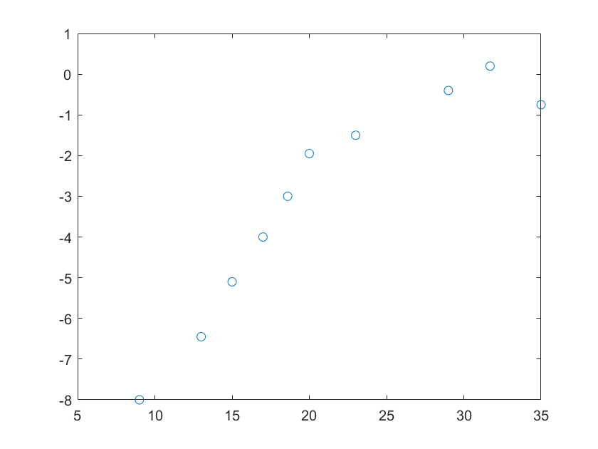
Draw discrete points

plot(x,y,'o')

Fit the above curve with a linear function

clear
clc
x=[12,9,23,56,43.5,33,41.3,76,63,26];
y=[-4,-3.85,-5.4,-5,-3.5,-1.75,-1.4,-0.5,0.4,-0.85];
coefficient=polyfit(x,y,1);  %Use a function to fit the curve. If you want to use several functions to fit the curve, set n to that number
y1=polyval(coefficient,x);
plot(x,y,'o',x,y1,'-')

result:

coefficient=[0.04603,-4.34700]

The one-time function obtained is:

y=0.04603x-4.34700

A quadratic function fits the curve, and the results are as follows:

coefficient=[2.29779e-04,0.02709,-4.05811]

Other orders by analogy

The number m of non-repetitive elements in the vector x (with elements as independent variables) and the fitting order k need to satisfy m>=k+1. Simple analysis: k-order fitting needs to determine k+1 unknown parameters (such as The first-order fitting y = ax + b needs to determine the two parameters a and b), so at least k+1 equations are required, so at least k+1 different known number pairs (x, y) are required, because the function x can only correspond to one y, so at least k+1 different x is required.

For example, it is normal to fit the above curve with a 9th-order polynomial.

Fit the above curve with a tenth-order polynomial, and get incorrect results:

Original link jab
WeChat gongzhonghao: Optimized algorithm exchange

Intelligent Recommendation

Linear least squares method (with MATLAB code)

This article is partially reproducedOptimization algorithm exchangeText, reprint only works. Give a given data with N times polynomial. Note: For nonlinear curves, such as index curves\(y=a_{1}e^{a_{2...

MATLAB to achieve the least squares method of curve fitting

Experimental conditions Experimental case x 0 10 20 30 40 50 60 70 80 90 y 68 67.1 66.4 65.6 64.6 61.8 61.0 60.8 60.4 60 Experimental requirements The approximate value of the approximation function f...

Python implements least squares method for linear fitting

Fundamental The least square method (also known as the least square method) is a mathematical optimization technique. It finds the best function match of the data by minimizing the sum of squares of e...

MATLAB implements least square method

Article Source: The least square method (also known as the least square method) is a mathematical optimization technique. It finds the best function match of the data by minimizing the sum of squares ...

Matlab least squares fitting

Nonlinear fitting Here is an example of fitting year and population The year increases in ten-year intervals from 1790-2000. The specific code is as follows: result: xsim = 1 to 14 columns 15 to 24 co...