table of Contents

0 principle    1 For example    1) Binarization    2) Remove all white noise in the image   3) Extract the area that is definitely a coin   4) Obtain the boundary area

5) Marked area   6) Implement the watershed algorithm

---

0 principle

In geography, a watershed is a ridge that distinguishes drainage areas by different water systems. A catchment basin is a geographical area where water is discharged into a river or reservoir. The watershed transform applies these concepts to grayscale image processing to solve many image segmentation problems.

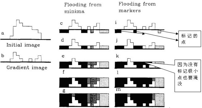
Understanding the watershed transform requires that we consider the grayscale image as a topological surface, and the value of f(x, y) in the surface is interpreted as height. For example, we can visualize the simple image in (a) below as the three-dimensional surface in (b) below. If rainwater falls on the surface, the rain will obviously flow into the two catchment basins. Rainwater that just landed on the watershed ridge will flow equally into the two catchment basins. The watershed transform will find the catchment basin and ridgeline in the grayscale image. In solving the problem of image segmentation, the key concept is to change the starting image into another image. In the transformed image, the catchment basin is the object or region we want to identify.

OpenCV uses a mask-based watershed algorithm, in which we set up those valley points to meet, and those that don't. This is an interactive image segmentation. We have to do is give us the known objects marked with different labels. If an area is definitely a foreground or object, mark it with a color (or gray value) label. If an area is definitely not an object but the background is marked with another color label. The rest of the area that cannot be determined to be foreground or background is marked with 0. This is our label. Then implement the watershed algorithm. Each time we fill, our label is updated. When two different colored labels meet, we build the dam until all the peaks are submerged. Finally we get the boundary object (dam) with a value of -1.

1 Example

First look at the following example, and then explain the meaning inside:

1) Binarization

We start by finding an approximate estimate of the coin. We can use Otsu's binarization.

import numpy as np
import cv2
from matplotlib import pyplot as plt

src = cv2.imread('test27.jpg')
img = src.copy()
gray = cv2.cvtColor(img, cv2.COLOR_BGR2GRAY)
ret, thresh = cv2.threshold(
    gray, 0, 255, cv2.THRESH_BINARY_INV+cv2.THRESH_OTSU)

2) Remove all white noise in the image

This requires the use of open operations in morphology. In order to remove small holes in the object we need to use a morphological closing operation. So we now know that the area near the center of the object is definitely the foreground, and the area far from the center of the object is definitely the background. The area that cannot be determined is the boundary between coins.

kernel = np.ones((3, 3), np.uint8)
opening = cv2.morphologyEx(thresh, cv2.MORPH_OPEN, kernel, iterations=2)

Open operation can refer to:

3) Extract the area that is definitely a coin

a. When there is no contact between the coins

Corrosion operations remove edge pixels. The rest is definitely a coin.

b. The coins are in contact with each other

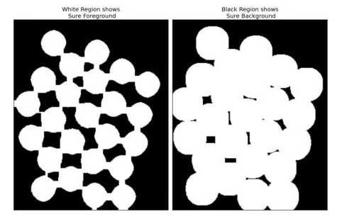
The distance transform plus the appropriate threshold. Next we have to find an area that is definitely not a coin. This is the need for expansion operations. Swelling extends the boundaries of the object into the background. So because the boundary areas are processed, we can know that those areas are definitely foreground, and those are definitely the background.

# 
sure_bg = cv2.dilate(opening, kernel, iterations=3)

 # 
dist_transform = cv2.distanceTransform(opening, 1, 5)
ret, sure_fg = cv2.threshold(dist_transform, 0.7*dist_transform.max(), 255, 0)

Expansion operation can refer to:

        

Distance transformation function:

cv2.distanceTransform(src, distanceType, maskSize)

• src：Input image
• distanceType：The way to calculate the distance, comes with 7 kinds

                        DIST_L1      = 1,   //!< distance = |x1-x2| + |y1-y2|

                        DIST_L2      = 2,   //!< the simple euclidean distance

                        DIST_C       = 3,   //!< distance = max(|x1-x2|,|y1-y2|)

                        DIST_L12     = 4,   //!< L1-L2 metric: distance = 2(sqrt(1+x*x/2) - 1))

                        DIST_FAIR    = 5,   //!< distance = c^2(|x|/c-log(1+|x|/c)), c = 1.3998

                        DIST_WELSCH  = 6,   //!< distance = c^2/2(1-exp(-(x/c)^2)), c = 2.9846

                        DIST_HUBER   = 7    //!< distance = |x|<c ? x^2/2 : c(|x|-c/2), c=1.345

• maskSize：Mask size, 3 types

                        DIST_MASK_3 = 3, //!< mask=3

                        DIST_MASK_5 = 5, //!< mask=5

                        DIST_MASK_PRECISE = 0 //!< mask=0

4) Obtain the boundary area

The rest of the area is that we don't know how to distinguish. This is what the watershed algorithm does. These areas are usually the junction of the foreground and the background (or the junction of the two foregrounds). We call it the border.

sure_fg = np.uint8(sure_fg)
unknown = cv2.subtract(sure_bg, sure_fg)

5) Marked area

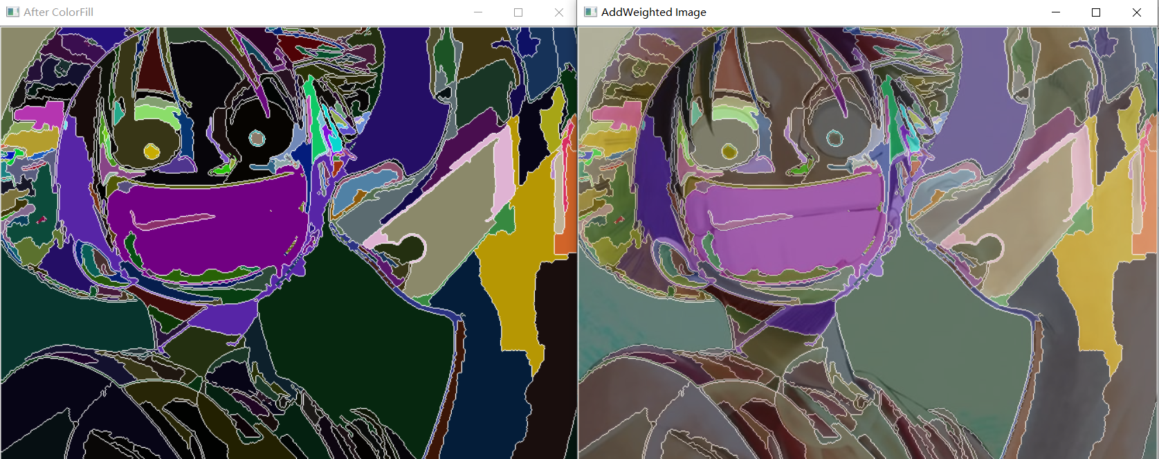
Now I know that those are the backgrounds that are coins. Then we can create a label (an array of the same size as the original image, the data type is in32) and mark the area. Use a different positive integer mark for the area we have identified (whether foreground or background) and a 0 mark for areas we don't know. We can do this using the function cv2.connectedComponents() . It marks the background as 0, and other objects use a positive integer token starting at 1. However, we know that if the background marker is 0, then the watershed algorithm will treat it as an unknown region. So we want to mark them with different integers. The area that is indeterminate (the unknown is defined in the result of the function cv2.connectedComponents output is unknown) is marked as 0.

# 
ret, markers1 = cv2.connectedComponents(sure_fg)

 # Make sure the background is 1 is not 0
markers = markers1 + 1

 # Unknown area marked as 0
markers[unknown == 255] = 0

The result is represented using a JET color map. The dark blue area is an unknown area. The area of ​​the coin must be marked with a different color. The rest of the area is the background marked in light blue.

Where the connectedComponents() function:

cv2.connectedComponents(image, labels, connectivity, ltype)

• image：Enter 8-bit single channel image
• labels：Output tag map
• connectivity：Connectivity, default 8, can also take 4
• ltype：Output tag type, default CV_32S, can also take CV_16U

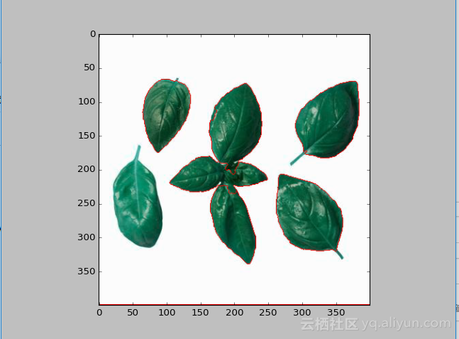
6) Implement the watershed algorithm

The label image will be modified and the marker in the border area will change to -1

markers3 = cv2.watershed(img, markers)
img[markers3 == -1] = [0, 0, 255]

The watershed algorithm function:

cv2.watershed(img, markers)

• img：Input image
• markers：mark

Finally all the procedures are as follows:

import numpy as np
import cv2
from matplotlib import pyplot as plt

src = cv2.imread('test27.jpg')
img = src.copy()
gray = cv2.cvtColor(img, cv2.COLOR_BGR2GRAY)
ret, thresh = cv2.threshold(
    gray, 0, 255, cv2.THRESH_BINARY_INV+cv2.THRESH_OTSU)

# Eliminate noise
kernel = np.ones((3, 3), np.uint8)
opening = cv2.morphologyEx(thresh, cv2.MORPH_OPEN, kernel, iterations=2)

 # 
sure_bg = cv2.dilate(opening, kernel, iterations=3)

 # 
dist_transform = cv2.distanceTransform(opening, 1, 5)
ret, sure_fg = cv2.threshold(dist_transform, 0.7*dist_transform.max(), 255, 0)

 #Get an unknown area
sure_fg = np.uint8(sure_fg)
unknown = cv2.subtract(sure_bg, sure_fg)

 # 
ret, markers1 = cv2.connectedComponents(sure_fg)

 # Make sure the background is 1 is not 0
markers = markers1 + 1

 # Unknown area marked as 0
markers[unknown == 255] = 0

markers3 = cv2.watershed(img, markers)
img[markers3 == -1] = [0, 0, 255]

plt.subplot(241), plt.imshow(cv2.cvtColor(src, cv2.COLOR_BGR2RGB)),
plt.title('Original'), plt.axis('off')
plt.subplot(242), plt.imshow(thresh, cmap='gray'),
plt.title('Threshold'), plt.axis('off')
plt.subplot(243), plt.imshow(sure_bg, cmap='gray'),
plt.title('Dilate'), plt.axis('off')
plt.subplot(244), plt.imshow(dist_transform, cmap='gray'),
plt.title('Dist Transform'), plt.axis('off')
plt.subplot(245), plt.imshow(sure_fg, cmap='gray'),
plt.title('Threshold'), plt.axis('off')
plt.subplot(246), plt.imshow(unknown, cmap='gray'),
plt.title('Unknow'), plt.axis('off')
plt.subplot(247), plt.imshow(np.abs(markers), cmap='jet'),
plt.title('Markers'), plt.axis('off')
plt.subplot(248), plt.imshow(cv2.cvtColor(img, cv2.COLOR_BGR2RGB)),
plt.title('Result'), plt.axis('off')

plt.show()

The results are as follows: