ADMM, ISTA, Fista algorithm step detailed explanation, matlab code, solve the problem of Lasso optimization

Original article! Reprint need to indicate the source: ️ ️Sylvan Ding’s Blog ️

Purpose

• Understand the basic principles, convergence and complexity of ADMM, ISTA, FISTA algorithm;
• Use the above three algorithms to solve the lasso problem;
• Analyze the performance of the three algorithms.

lab environment

MATLAB R2021a

Experimental content

ADMM and [F] ISTA's convergence proof is given in [1] and [2], the global convergence rate of ADMM and ISTA O ( 1 / k ) O(1/k) O(1/k) [ECKSTEIN and Bertsekas, 1990; Deng and Yin, 2012; He and Yuan, 2012], but Fista's global convergence rate is O ( 1 / k 2 ) O(1/k^2) O(1/k2)Essence However, in some cases, ISTA concluded faster than Fista and gave specific reasons.

LASSO Problem

Many machine learning and data fitting problems can be regarded as the minimum secondary problem, adding regular items to avoid overfitting. In many applications, use l 1 l1 l1-For number as a regular item can bring a good generalization effect, so we solve l 1 l1 l1-The linear minimum secondary problem, also known as Lasso problem [2], the general form is: (P)

min ⁡ x ∈ R n 1 2 ∥ A x − b ∥ 2 + λ ∥ x ∥ 1 . \min \limits _{x\in \mathbb{R} ^n} \frac{1}{2} \Vert Ax-b \Vert ^2 + \lambda \Vert x \Vert _1. x∈Rnmin​21​∥Ax−b∥2+λ∥x∥1​.

in, A ∈ R m × n A\in \mathbb{R} ^{m\times n} A∈Rm×n It is a normal matrix, n > m n>m n>m ； b b b It is a known vector; λ > 0 \lambda >0 λ>0 It is a scalar; l 1 l1 l1-The regular item ∥ x ∥ 1 \Vert x \Vert _1 ∥x∥1​ A sparse solution will be produced, while reducing the cost, avoiding overfitting [Tibshirani, 1996].

existexperiment oneandExperiment threeAmong them, different regular items were used to achieve the noise reduction of the signal, which reflects l 1 l1 l1-In another advantage of the regular item is comparison l 2 l2 l2-The regular item, l 1 l1 l1-The regular item is not sensitive to the boundary value, which is conducive to the processing of Sharp Edges in the image noise reduction.

existExperiment threeIn the middle, the second optimization problem of Box-CONSTRAINED has been regarded as a second optimization problem, and the gradient projection method is solved. This article requires three algorithms such as ADMM, ISTA, and FISTA to solve the Lasso problem.

ADMM

Admm algorithm (Alternating Direction Method of Multipliers) x x x Decomptellerate to two variables x x x and z z z , Use in the minimum daily loss function x x x ,exist l 1 l1 l1-In the regular items of Fan Digital z z z Essence In this way, plus an equivalent constraint can construct a wide Laeglan daily function, and then solve the optimal value of the two variables separately, making it easier to calculate.

Question (p) equivalent at::

min ⁡ x 1 2 ∥ A x − b ∥ 2 + λ ∥ z ∥ 1 s . t . x − z = 0 \begin{array}{l} \min \limits _x & \frac{1}{2} \Vert Ax-b \Vert ^2 + \lambda \Vert z \Vert _1 \\ \mathrm{s.t.} & x-z=0 \end{array} xmin​s.t.​21​∥Ax−b∥2+λ∥z∥1​x−z=0​

Constructive Lagmeented Lagrangian L ρ L_\rho Lρ​ ：

L ρ ( x , z , μ ) = f ( x ) + g ( z ) + μ T ( x − z ) + ρ 2 ∥ x − z ∥ 2 . L_\rho (x,z,\mu) = f(x)+g(z)+\mu ^T(x-z) + \frac{\rho }{2} \Vert x-z \Vert ^2. Lρ​(x,z,μ)=f(x)+g(z)+μT(x−z)+2ρ​∥x−z∥2.

in, f ( x ) = 1 2 ∥ A x − b ∥ 2 f(x)=\frac{1}{2} \Vert Ax-b \Vert ^2 f(x)=21​∥Ax−b∥2 ， g ( z ) = λ ∥ z ∥ 1 g(z)=\lambda \Vert z \Vert _1 g(z)=λ∥z∥1​ ， ρ \rho ρ It is a punishment parameter.

It's not difficult to find, optimize x x x At this time, it is a second optimization problem, and the optimization z z z At this time, it is a Soft-Thresholding problem. Then, the iterative form of ADMM is:

x k + 1 : = ( A T A + ρ I ) − 1 ( A T b + ρ z k − μ k ) x . m i n i m i z a t i o n z k + 1 : = S λ / ρ ( x k + 1 + μ k / ρ ) z . m i n i m i z a t i o n μ k + 1 : = μ k + ρ ( x k + 1 − z k + 1 ) d u a l u p d a t e \begin{array}{l} x^{k+1} &:= (A^TA+\rho I)^{-1}(A^Tb+\rho z^k-\mu ^k) & \mathrm{ x.minimization } \\ z^{k+1} &:= S_{\lambda / \rho} (x^{k+1} + \mu ^{k}/ \rho) & \mathrm{ z.minimization }\\ \mu ^{k+1} &:= \mu ^k + \rho (x^{k+1}-z^{k+1}) & \mathrm{ dual \quad update } \end{array} xk+1zk+1μk+1​:=(ATA+ρI)−1(ATb+ρzk−μk):=Sλ/ρ​(xk+1+μk/ρ):=μk+ρ(xk+1−zk+1)​x.minimizationz.minimizationdualupdate​

in, S τ S_\tau Sτ​ It is a soft threshold function (also known as shrinkage), S τ ( g ) : = s i g n ( g ) ⋅ ( ∣ g ∣ − τ ) + S_\tau (g):=sign(g)\cdot (|g|-\tau)_+ Sτ​(g):=sign(g)⋅(∣g∣−τ)+​ [3], that is, [5]

[ S τ ( g ) ] j = { g j − τ g > τ 0 − τ ≤ g ≤ τ g j + τ g < − τ , j = 1 , 2 , … , n \left [S_\tau (g) \right ]_j= \left\{\begin{matrix} g_j-\tau & g> \tau \\ 0 & -\tau \le g \le \tau \\ g_j+\tau & g<-\tau \end{matrix}\right. , \quad j=1,2,\dots ,n [Sτ​(g)]j​=⎩⎨⎧​gj​−τ0gj​+τ​g>τ−τ≤g≤τg<−τ​,j=1,2,…,n

In fact, the ADMM algorithm can often get more accurate solutions after a series of iterations, but the number of iterations required is a large number [5].

ρ \rho ρ Selection will greatly affect the convergence of ADMM to a great extent. like ρ \rho ρ Too big, then for optimization f + g f+g f+g The ability will decline; on the contrary, it will weaken the constraint conditions x = z x=z x=z. Boyd et al. (2010) Give selection ρ \rho ρ The strategy is good, but it cannot guarantee that it must converge.

ISTA

A method of solving problems (P) is now ISTA (Iterates Shrinkage-Thresholding Algorithms) [Daubechies et al, 2004]. This method calculates the multiplication of matrix and vector at each iteration (shrinkage. /soft-threehold).

For continuous micro function f : R n → R f:\mathbb{R} ^n \to \mathbb{R} f:Rn→R No constraint optimization problem min ⁡ { f ( x ) : x ∈ R n } \min \{ f(x): x\in \mathbb{R} ^n \} min{f(x):x∈Rn} A simple way to solve such problems is to use gradient algorithms, pass x k = x k − 1 − t k ∇ f ( x k − 1 ) x_k=x_{k-1}-t_k\nabla f(x_{k-1}) xk​=xk−1​−tk​∇f(xk−1​) Generate { x k } \{ x_k \} {xk​}This gradient iteration method can be regarded as a linear function f f f Point x k − 1 x_{k-1} xk−1​ The proximal regulatory (proximal regulating) [Martinet, Bernard, 1970], that is

x k = arg ⁡ min ⁡ x { f ( x k − 1 ) + ⟨ x − x k − 1 , ∇ f ( x k − 1 ) ⟩ + 1 2 t k ∥ x − x k − 1 ∥ 2 } . x_k=\arg \min \limits _x \left \{ f(x_{k-1} ) + \left \langle x-x_{k-1},\nabla f(x_{k-1}) \right \rangle + \frac{1}{2t_k} \Vert x-x_{k-1} \Vert ^2 \right \}. xk​=argxmin​{f(xk−1​)+⟨x−xk−1​,∇f(xk−1​)⟩+2tk​1​∥x−xk−1​∥2}.

in, ⟨ x , y ⟩ = x T y \left \langle x,y \right \rangle =x^Ty ⟨x,y⟩=xTy Indicates the internal accumulation of the two vectors. Apply this gradient thought to non -smooth l 1 l1 l1-The optimization of regular items (P), then iteration strategies can be obtained:

x k = arg ⁡ min ⁡ x { f ( x k − 1 ) + ⟨ x − x k − 1 , ∇ f ( x k − 1 ) ⟩ + 1 2 t k ∥ x − x k − 1 ∥ 2 + λ ∥ x ∥ 1 } . x_k=\arg \min \limits _x \left \{ f(x_{k-1} ) + \left \langle x-x_{k-1},\nabla f(x_{k-1}) \right \rangle + \frac{1}{2t_k} \Vert x-x_{k-1} \Vert ^2 + \lambda \Vert x \Vert _1 \right \}. xk​=argxmin​{f(xk−1​)+⟨x−xk−1​,∇f(xk−1​)⟩+2tk​1​∥x−xk−1​∥2+λ∥x∥1​}.

After the same type, after ignoring the constant item, we can get the following form:

x k = arg ⁡ min ⁡ x { 1 2 t k ∥ x − ( x k − 1 − t k ∇ f ( x k − 1 ) ) ∥ 2 + λ ∥ x ∥ 1 } . x_k = \arg \min \limits _x \left \{ \frac{1}{2t_k} \Vert x-(x_{k-1}-t_k\nabla f(x_{k-1})) \Vert ^2 + \lambda \Vert x \Vert _1 \right \}. xk​=argxmin​{2tk​1​∥x−(xk−1​−tk​∇f(xk−1​))∥2+λ∥x∥1​}.

This is a special situation, because l 1 l1 l1-Fan number can be separated, so calculation x k x_k xk​ Simplify to solve the problem of one -dimensional optimization, that is,

x k = τ λ t k ( x k − 1 − t k ∇ f ( x k − 1 ) ) . x_{k}=\tau _{\lambda t_k} (x_{k-1} -t_k\nabla f(x_{k-1})). xk​=τλtk​​(xk−1​−tk​∇f(xk−1​)).

When for the (P) problem, the iterative form of ISTA is: ( P i s t a P_{ista} Pista​）

x k + 1 = τ λ t k + 1 ( x k − t k + 1 A T ( A x k − b ) ) . x_{k+1}=\tau _{\lambda t_{k+1}} (x_k -t_{k+1}A^T(Ax_k-b)). xk+1​=τλtk+1​​(xk​−tk+1​AT(Axk​−b)).

in, t k + 1 t_{k+1} tk+1​ For steppae t k ∈ ( 0 , 1 / ∥ A T A ∥ ) t_k\in (0,1/\Vert A^TA \Vert ) tk​∈(0,1/∥ATA∥) Ensured x k x_k xk​ Can converge x ∗ x^* x∗ 。 τ α \tau _{\alpha} τα​It is the same as Shrinkage Operator, which is no different from the shrinkage function. [1] Proved decline and convergence.

The idea of ​​this algorithm can be traced back to the Pro Ximal FORAWARDBACKWARD ITERATIVE Scheme. Recently, a proximal forward-backward algorithms { x k } \{ x_k \} {xk​} The algorithm of the sequence also contributed [1].

for( P i s t a P_{ista} Pista​), Bobe t t t There are two ways to determine, namely the fixed steps and the backtracking method. When using the fixed step length, we need to set t ˉ = 1 / L ( f ) \bar{t}=1/L(f) tˉ=1/L(f) ， L ( f ) L(f) L(f) yes ∇ f \nabla f ∇f Lipschitz constant. For (P), L ( f ) = 2 λ max ⁡ ( A T A ) L(f)=2\lambda _{\max} (A^TA) L(f)=2λmax​(ATA) This leads to large -scale problems ( A A A The number of dimensions is too large), solve L ( f ) L(f) L(f) It is often difficult, and many times, L ( f ) L(f) L(f) Can't find it. Therefore, we use the retrospective method to solve the right step. (R)

Although ISTA is a very simple method, its convergence speed is slower. Recent studies have shown that for some specific ones A A A , ISTA generated { x k } \{ x_k \} {xk​} The sequence has the same slowly gradual convergence rate, which is bad [bredies and d. Lorenz, 2008].

FISTA

So, now it is necessary to find an algorithm as simple as ISTA, but it is better than ISTA in terms of speed. Beck a, Teboulle M τ \tau τ Useless x k − 1 x_{k-1} xk−1​ On it, but use it y k y_k yk​ superior, y k y_k yk​ In combination with a linear way x k − 1 x_{k-1} xk−1​ and x k − 2 x_{k-2} xk−2​ ,Right now

x k = τ λ / L k ( y k − 1 L k A T ( A y k − b ) ) x_{k}=\tau _{\lambda /L_{k}} (y_k -\frac{1}{L_k}A^T(Ay_k-b)) xk​=τλ/Lk​​(yk​−Lk​1​AT(Ayk​−b))

y k + 1 = x k + ( t k − 1 t k + 1 ) ( x k − x k − 1 ) . y_{k+1}=x_k+\left ( \frac{t_k-1}{t_{k+1}} \right )(x_k - x_{k-1}). yk+1​=xk​+(tk+1​tk​−1​)(xk​−xk−1​).

also, t k t_k tk​ The iterative strategy is:

t k + 1 = 1 + 1 + 4 t k 2 2 . t_{k+1}=\frac{1+\sqrt{1+4t^2_k}}{2}. tk+1​=21+1+4tk2​ ​​.

Attention, here t k + 1 t_{k+1} tk+1​ Not a step, but y k + 1 y_{k+1} yk+1​ The coefficient of linear combination of the previous two iteration results. The step is at this time L L L ， L L L It happens to be the countdown with the previous steps. Same as the above reasons (R), we also use the retrospective method to solve the right step.

Algorithm Description

ADMM

ADMM Algorithm for LASSO problem based on [4-5]

% Solves the following problem via ADMM:
% minimize 1/2*|| Ax - b ||_2^2 + \lambda || x ||_1

% INPUT
%=======================================
% A
% b
% rho ....... augmented Lagrangian parameter
% lambda .... coefficient of l1-norm
% iter ...... iteration number
% OUTPUT
%=======================================
% x_s ....... sequences {xk} generated by ADMM

1. Initialization x 0 , z 0 , μ 0 = 0 x_0,z_0,\mu _0 = \mathrm{0} x0​,z0​,μ0​=0 [6]
2. Update variables ( k ≥ 0 k \ge 0 k≥0）：

x k + 1 : = ( A T A + ρ I ) − 1 ( A T b + ρ z k − μ k ) x . m i n i m i z a t i o n z k + 1 : = S λ / ρ ( x k + 1 + μ k / ρ ) z . m i n i m i z a t i o n μ k + 1 : = μ k + ρ ( x k + 1 − z k + 1 ) d u a l u p d a t e \begin{array}{l} x^{k+1} &:= (A^TA+\rho I)^{-1}(A^Tb+\rho z^k-\mu ^k) & \mathrm{ x.minimization } \\ z^{k+1} &:= S_{\lambda / \rho} (x^{k+1} + \mu ^{k}/ \rho) & \mathrm{ z.minimization }\\ \mu ^{k+1} &:= \mu ^k + \rho (x^{k+1}-z^{k+1}) & \mathrm{ dual \quad update } \end{array} xk+1zk+1μk+1​:=(ATA+ρI)−1(ATb+ρzk−μk):=Sλ/ρ​(xk+1+μk/ρ):=μk+ρ(xk+1−zk+1)​x.minimizationz.minimizationdualupdate​

[F]ISTA

[F]ISTA with backtracking for LASSO problem based on [1]

% Solves the following problem via [F]ISTA:
% minimize 1/2*|| Ax - b ||_2^2 + \lambda || x ||_1

% INPUT
%=======================================
% A
% b
% x0......... initial point
% L0 ........ initial choice of stepsize
% eta ....... the constant in which the stepsize is multiplied
% lambda .... coefficient of l1-norm
% iter ...... iteration number
% opt ....... 0 for ISTA or 1 for FISTA
% eps ....... stop criterion
% OUTPUT
%=======================================
% x_s ....... sequences {xk} generated by [F]ISTA

1. Pick L 0 > 0 , η > 1 , x 0 ∈ R n L_0>0 ,\eta>1,x_0 \in \mathbb{R} ^n L0​>0,η>1,x0​∈Rn, set up y 1 = x 0 , t 1 = 1 y_1=x_0,t_1=1 y1​=x0​,t1​=1 ;

2. First k ≥ 1 k \ge 1 k≥1 Step, look for the minimum non -negative integer i k i_k ik​ , Make L ˉ = η i k L k − 1 \bar{L}=\eta ^{i_k}L_{k-1} Lˉ=ηik​Lk−1​, have
   F ( p L ˉ ( y k ) ) ≤ Q L ˉ ( p L ˉ ( y k ) , y k ) . F(p_{\bar{L}}(y_k))\le Q_{\bar{L}} (p_{\bar{L}}(y_k), y_k). F(pLˉ​(yk​))≤QLˉ​(pLˉ​(yk​),yk​). [1]

   in,

   F ( x ) ≡ f ( x ) + g ( x ) , F(x) \equiv f(x)+g(x), F(x)≡f(x)+g(x),

   ∇ f ( y ) = A T ( A y − b ) , \nabla f(y) = A^T(Ay-b) , ∇f(y)=AT(Ay−b),

   p L ˉ ( y k ) = τ λ / L ˉ ( y k − 1 L ˉ A T ( A y k − b ) ) , p_{\bar{L}} (y_k) = \tau _{\lambda /\bar{L}} (y_k -\frac{1}{\bar{L}}A^T(Ay_k-b)) , pLˉ​(yk​)=τλ/Lˉ​(yk​−Lˉ1​AT(Ayk​−b)),

   Q L ˉ ( x , y ) : = f ( y ) + ⟨ x − y , ∇ f ( y ) ⟩ + L ˉ 2 ∥ x − y ∥ 2 + g ( x ) . Q_{\bar{L}}(x,y):=f(y)+\left \langle x-y,\nabla f(y) \right \rangle + \frac{\bar{L}}{2} \Vert x-y \Vert ^2 + g(x) . QLˉ​(x,y):=f(y)+⟨x−y,∇f(y)⟩+2Lˉ​∥x−y∥2+g(x).

3. set up L k = η i k L k − 1 L_k=\eta ^{i_k} L_{k-1} Lk​=ηik​Lk−1​ , Update the following variables: [2]

   x k = p L k ( y k ) , x_{k}= p_{L_k} (y_k), xk​=pLk​​(yk​),

   t k + 1 = 1 + 1 + 4 t k 2 2 , t_{k+1}=\frac{1+\sqrt{1+4t^2_k}}{2}, tk+1​=21+1+4tk2​ ​​,

   δ k = 0   f o r   I S T A ,   o r   t k − 1 t k + 1   f o r   F I S T A , \delta _k=0 \ \mathrm{for \ ISTA},\ or\ \frac{t_k-1}{t_{k+1}}\ \mathrm{for \ FISTA}, δk​=0 for ISTA, or tk+1​tk​−1​ for FISTA,

   y k + 1 = x k + δ k ( x k − x k − 1 ) . y_{k+1} = x_{k} + \delta _k (x_k-x_{k-1}) . yk+1​=xk​+δk​(xk​−xk−1​).

Note:Remark 3.2 [1] Give it L k L_k Lk​ Range range:

L 0 ≤ L k ≤ η L ( f ) . L_0\le L_k \le \eta L(f) . L0​≤Lk​≤ηL(f).

Experimental step

set up m = 1500 , n = 5000 , p = 0.02 m=1500,n=5000,p=0.02 m=1500,n=5000,p=0.02 ， p p p It's true u u u Sparsy density, A ∈ R m × n A\in \mathbb{R} ^{m\times n} A∈Rm×n. b = A*u + sqrt(0.001)*randn(m,1); exist b b b Added random noise, initial value x 0 = 0 x_0=0 x0​=0 ， λ = 0.15 \lambda=0.15 λ=0.15 Evestation of errors E ( x ^ ) = ∥ x ^ − u ∥ 1 E(\hat{x}) = \Vert \hat{x}-u \Vert _1 E(x^)=∥x^−u∥1​ ， x ^ \hat{x} x^ It is a predicted value.

clc;clear

randn('seed', 0);
rand('seed',0);

m = 1500;       % number of examples
n = 5000;       % number of features
p = 100/n;      % sparsity density

u = sprandn(n,1,p);
A = randn(m,n);
A = A*spdiags(1./sqrt(sum(A.^2))',0,n,n); % normalize columns
b = A*u + sqrt(0.001)*randn(m,1);

iter = 70;
lambda = 0.15;
x0 = zeros(5000,1);

E = @(x) sum(abs(x-u)); % compute error

ADMM [6]

set up ρ = 0.7 \rho = 0.7 ρ=0.7 .

%% ADMM DEMO
rho = 0.7;
x_admm = admm_lasso(A,b,rho,lambda,iter);
conv_admm = E(x_admm);

function x_s = admm_lasso(A,b,rho,lambda,iter)
% Solves the following problem via ADMM:
% minimize 1/2*|| Ax - b ||_2^2 + \lambda || x ||_1

% INPUT
%=======================================
% A
% b
% rho ....... augmented Lagrangian parameter
% lambda .... coefficient of l1-norm
% iter ...... iteration number
% OUTPUT
%=======================================
% x_s ....... sequences {xk} generated by ADMM

%% shrinkage operator
S = @(tau, g) max(0, g - tau) + min(0, g + tau);

x_s = [];
[~,n] = size(A);
I = eye(n);
x = zeros(n,1);
z_old = zeros(n,1);
u_old = zeros(n,1);
%% MAIN LOOP
for ii = 1:iter
    % record x_s
    x_s = [x_s, x];
    % minimize x,z,u
    x = (A'*A+rho*I) \ (A'*b+rho*z_old-u_old);
    z_new = S(lambda/rho, x+u_old/rho);
    u_new = u_old + rho*(x-z_new);
    % check stop criteria
    % e = norm(x_new-x_old,1)/numel(x_new);
    % if e < eps
        % break
    % end
    % update
    z_old = z_new;
    u_old = u_new;
end

[F]ISTA [7]

set up L 0 = 1.05 , η = 1.01 L_0=1.05,\eta=1.01 L0​=1.05,η=1.01 .

%% [F]ISTA DEMO
L0 = 1.05;
eta = 1.01;
x_ista = fista_backtracking_lasso(A,b,x0,L0,eta,lambda,iter,0,0);
conv_ista = E(x_ista);
x_fista = fista_backtracking_lasso(A,b,x0,L0,eta,lambda,iter,1,0);
conv_fista = E(x_fista);

function x_s = fista_backtracking_lasso(A,b,x0,L0,eta,lambda,iter,opt, eps)
% Solves the following problem via [F]ISTA:
% minimize 1/2*|| Ax - b ||_2^2 + \lambda || x ||_1

% INPUT
%=======================================
% A
% b
% x0......... initial point
% L0 ........ initial choice of stepsize
% eta ....... the constant in which the stepsize is multiplied
% lambda .... coefficient of l1-norm
% iter ...... iteration number
% opt ....... 0 for ISTA or 1 for FISTA
% eps ....... stop criterion
% OUTPUT
%=======================================
% x_s ....... sequences {xk} generated by [F]ISTA

%% f = 1/2*|| Ax - b ||_2^2
f = @(x) 0.5 * norm(A*x-b)^2;

%% g = \lambda || x ||_1
g = @(x) lambda * norm(x,1);

%% the gradient of f
grad = @(x) A'*(A*x-b);

%% computer F
F = @(x) 0.5*(norm(A*x-b))^2 + lambda*norm(x,1);

%% shrinkage operator
S = @(tau, g) max(0, g - tau) + min(0, g + tau);

%% projection
P = @(L, y) S(lambda/L, y - (1/L)*grad(y));

%% computer Q
Q = @(L, x, y) f(y) + (x-y)'*grad(y) + 0.5*L*norm(x-y) + g(x);

x_s = [];
x_old = x0;
y_old = x0;
L_new = L0;
t_old = 1;
%% MAIN LOOP
for ii = 1:iter
    % find i_k
    j = 1;
    while true
        L_bar = eta^j * L_new;
        if F(P(L_bar, y_old)) <= Q(L_bar, P(L_bar, y_old), y_old)
            L_new = L_new * eta^j;
            break
        else
            j = j + 1;
        end
    end
    x_new = P(L_new, y_old);
    t_new = 0.5 * (1+sqrt(1+4*t_old^2));
    del = opt * (t_old-1)/(t_new);
    y_new = x_new + del*(x_new-x_old);
    % record x_s
    x_s = [x_s, x_new];
    % check stop criteria
    % e = norm(x_new-x_old,1)/numel(x_new);
    % if e < eps
        % break
    % end
    % update
    x_old = x_new;
    t_old = t_new;
    y_old = y_new;
end

Note: Here is a combination of ISTA and Fista algorithms into one, and OPT parameters can be selected. In the function, the stop condition is addedcheck stop criteria, For the convenience of testing, it is not used here, so it is released.

Draw

%% draw
plot(conv_admm,'LineWidth',1,...
    'DisplayName','ADMM','Color','black')
hold on
plot(conv_ista,'--','LineWidth',1,...
    'DisplayName','ISTA','Color','blue')
plot(conv_fista,'-.','LineWidth',1,...
    'DisplayName','FISTA','Color','red')
hold off
ylim([0 270])
xlabel('iteration k')
ylabel('$E(\bar{x})$','Interpreter','latex')
legend('Location','northeast')
title('Convergence behavior in terms of error of iterates of ADMM, ISTA, FISTA.',...
    '$m=1500,n=5000,p=0.02,x_0=0,\lambda=0.15,\rho = 0.7,L_0=1.05,\eta=1.01$',...
    'Interpreter','latex')

Result analysis

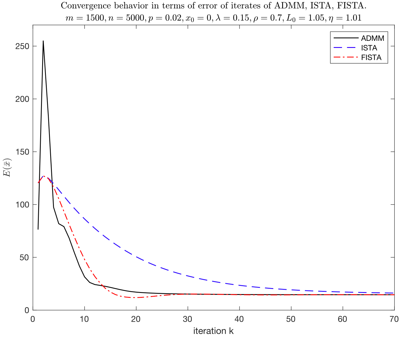
In this experiment, the convergence rate of the ADMM algorithm is the fastest. The convergence speed of FISTA is comparable to that of ADMM, and ISTA is the slowest. In ADMM, set ρ = 0.7 \rho = 0.7 ρ=0.7 ， ρ \rho ρ Small, although it has obtained a good convergence rate, it may weaken the constraints to a certain extent x = z x=z x=zIn addition, ADMM at the second iteration (all methods exist in this problem, for the time being unclear), E ( x ˉ ) E(\bar{x}) E(xˉ) The fluctuation range is large. In addition, the convergence rate of Fista is significantly better than ISTA. At about 20 iterations, the best value reached.

During the experiment, the ADMM solution speed is significantly slower than ISTA and FISTA. The main consumption of time is calculation x k + 1 x_{k+1} xk+1​ Time to reverse operations.

Original article! Reprint need to indicate the source: ️ ️Sylvan Ding’s Blog ️

references

1. Beck A, Teboulle M. A fast iterative shrinkage-thresholding algorithm for linear inverse problems[J]. SIAM journal on imaging sciences, 2009, 2(1): 183-202.
2. Tao S, Boley D, Zhang S. Convergence of common proximal methods for l1-regularized least squares[C]//Twenty-Fourth International Joint Conference on Artificial Intelligence. 2015.
3. Selesnick I. A derivation of the soft-thresholding function[J]. Polytechnic Institute of New York University, 2009.
4. S. Boyd. Alternating Direction Method of Multipliers. Available online at https://web.stanford.edu/class/ee364b/lectures/admm_slides.pdf.
5. Ryan Tibshirani. Alternating Direction Method of Multipliers. Available online at https://stat.cmu.edu/~ryantibs/convexopt/lectures/admm.pdf.
6. You are allowed to develop your solvers by adopting the ADMM codes available from the following Stanford University websites: https://web.stanford.edu/~boyd/papers/admm/lasso/lasso.html.
7. Tiep Vu. fista_backtracking.m. Available online at https://github.com/tiepvupsu/FISTA.