Soft threshold iteration algorithm (ISTA) and fast soft threshold iteration algorithm (FISTA)
tags: Compressed sensing
If the moon is missing, you will hang out the trees, and you will be quiet.
Who sees Youren coming and going alone, lonely and lonely.
was shocked but turned around, hate nobody.
Picking up the cold branches and refusing to perch, the lonely sandbar is cold. ---- Su Shi
For more exciting content, please follow the WeChat public account "Optimization and algorithm”
The ISTA algorithm and the FISTA algorithm are classic methods for solving linear inverse problems. They belong to the gradient algorithm and are also often used in the compressed sensing reconstruction algorithm. They belong to the gradient algorithm. This time, the principles of the two algorithms are briefly analyzed and given A matlab simulation experiment was used to verify the performance of the algorithm through the experimental results.
1 Introduction
For a basic linear inverse problem:
among them
,
And is known,
Is unknown noise.
(1) The formula can be solved by Least Squares:
when And When it is not singular, the solution of the least square method is equivalent to 。
However, in many cases, It is ill-conditioned. At this time, when the least squares method is used to solve the problem, the small disturbance of the system will cause the results to be very different, which can be described as ill-conditioned. Therefore, the least squares method is not suitable for solving ill-conditioned equations.
**What is the condition number? ** Matrix The condition number refers to The ratio of the largest singular value to the smallest singular value of, obviously the minimum condition number is 1. The smaller the condition number, the more the matrix tends to be "good", the larger the condition number, the more the matrix tends to be singular.
In order to solve the inverse problem of ill-conditioned linear systems, the former Soviet Union scientist Andrei Nikolayevich Tikhonov proposed the Tikhonov regularization method (Tikhonov regularization), which is also called "ridge regression" . Least squares is an unbiased estimation method (very good fidelity). If the system is ill-conditioned, it will lead to a large estimation variance (sensitive to disturbances). The main idea of Tikhonov's regularization method is A tolerable small deviation is exchanged for good estimation results, and a trade-off of variance and deviation is realized. Tikhonov's regularization to solve the ill-conditioned problem can be expressed as:
among them
It is a regularization parameter. The solution of problem (3) is equivalent to the following ridge regression estimator:
Andrei Nikolayevich Tikhonov (Russian: Alvald Pleyeva; October 17, 1906 to October 7, 1993 Japan) is a Soviet and Russian mathematician and geophysicist, known for his important contributions to topology, functional analysis, mathematical physics and ill-posed problems. He is also one of the inventors of the magnetotelluric method in geophysics.
Ridge regression is adopted
The norm is used as a regular term. Another way to solve equation (1) is to use
Norm as a regular term, this is the classicLASSO(Least absolute shrinkage and selection operator) question:
Adopt The norm regular term is relative to The norm regular term has two advantages, the first advantage is The norm regular term can produce sparse solutions. The second advantage is that it is insensitive to outliers, which is the opposite of ridge regression.
The problem in equation (5) is a convex optimization problem, which can usually be transformed into a second-order cone programming problem, which can be solved by methods such as interior point. However, in large-scale problems, due to the large data dimension, the algorithm complexity of the interior point method is , Resulting in a very time-consuming solution.
For the above reasons, many researchers have studied to solve equation (5) through a simple gradient-based method. The calculation amount of the gradient-based method is mainly concentrated in the matrix With vector In terms of the product of, the algorithm complexity is small, and the algorithm structure is simple and easy to operate.
2. Iterative Shrinkage Threshold Algorithm (ISTA)
Among many gradient-based algorithms, iterative shrinkage threshold algorithm (Iterative Shrinkage Thresholding Algorithm) is a very interesting algorithm. The ISTA algorithm is updated through a shrinkage/soft threshold operation in each iteration
, The specific iteration format is as follows:
among them
Is the soft threshold operation function:
The soft threshold operation function is shown in the figure below:
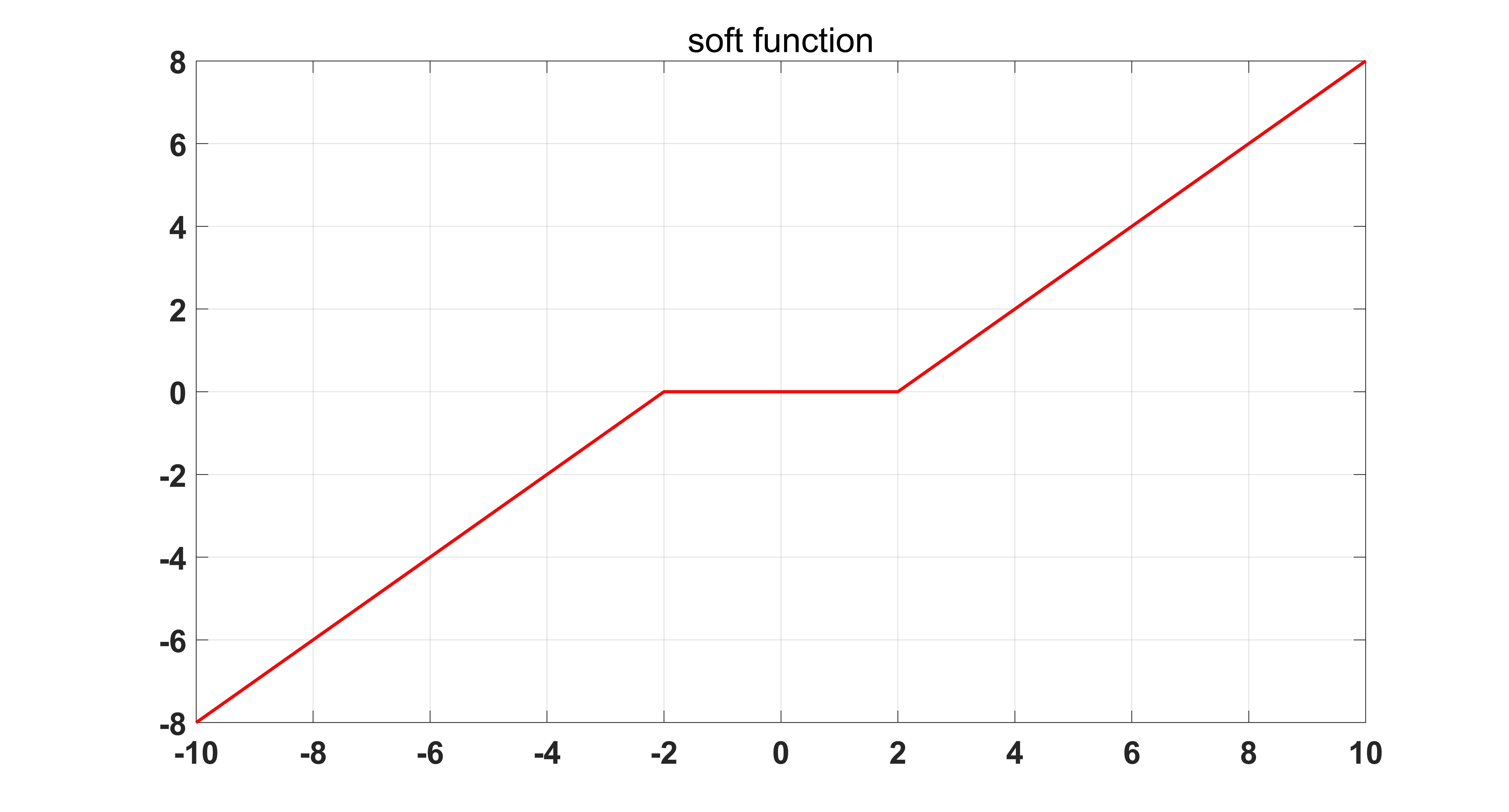
where
Is a symbolic function.
So how did the iterative format (6) of ISTA come from? Where is the "shrinkage threshold" in the algorithm? This starts with the gradient descent method (Gradient Descent).
Consider a continuous and derivable unconstrained minimization problem:
(8) Equation can be solved by gradient descent method:
Here
Is the iteration step. We know that the gradient descent method can be expressed as
At the point
Proximal regularization at, its equivalent form can be expressed as:
(9)-(10) The Lipschitz continuous condition with In The second-order Taylor expansion at the position is very simple, so I won’t repeat it here.
Add (8)
Norm regular term, we get:
Then (10) correspondingly becomes:
When (12) ignore the constant term
with
After that, (12) can be written as:
It has been proved in the literature that when the iteration step The reciprocal of Lipschitz constant (ie ), the sequence generated by the ISTA algorithm The convergence rate is , Is obviously the sub-linear convergence rate.
See the original text for the pseudo code of the ISTA algorithm, and the matlab code is as follows:
function [x_hat,error] = cs_ista(y,A,lambda,epsilon,itermax)
% Iterative Soft Thresholding Algorithm(ISTA)
% Version: 1.0 written by Louis Zhang @2019-12-7
% Reference: Beck, Amir, and Marc Teboulle. "A fast iterative
% shrinkage-thresholding algorithm for linear inverse problems."
% SIAM journal on imaging sciences 2.1 (2009): 183-202.

% Inputs:
% y         - measurement vector
% A         - measurement matrix
% lambda    - denoiser parameter in the noisy case
% epsilon   - error threshold
% inter_max - maximum number of amp iterations
%
% Outputs:
% x_hat     - the last estimate
% error     - reconstruction error

if nargin < 5
    itermax = 10000 ;
end
if nargin < 4
    epsilon = 1e-4 ;
end
if nargin < 3
    lambda = 2e-5 ;
end

N = size(A,2) ;
error = [];
x_1 = zeros(N,1) ;

for i = 1:itermax
    g_1 = A'*(y - A*x_1) ;
    alpha = 1 ;
    % obtain step size alpha by line search
    % alpha = (g_1'*g_1)/((A*g_1)'*(A*g_1)) ;
    x_2 = x_1 + alpha * g_1 ;
    x_hat = sign(x_2).*max(abs(x_2)-alpha*lambda,0) ;
    error(i,1) = norm(x_hat - x_1) / norm(x_hat) ;
    error(i,2) = norm(y-A*x_hat) ;
    if error(i,1) < epsilon || error(i,1) < epsilon
        break;
    else
        x_1 = x_hat ;
    end
end
In the actual process, the matrix It is usually very large and it is very difficult to calculate its Lipschitz constant. Therefore, a Backtracking version of the ISTA algorithm appears, which converges by continuously shrinking the iteration step.
3. Fast Iterative Shrinkage Thresholding Algorithm (FISTA)
In order to accelerate the convergence of the ISTA algorithm, the author in the literature uses a famous gradient acceleration strategyNesterov acceleration technology, Which makes the convergence speed of the ISTA algorithm change from Become . The specific proof process can be found in Theorem 4.1 of the original text.
Compared with the ISTA algorithm, FISTA only has one more Nesterov acceleration step, which greatly improves the convergence speed of the algorithm with very little additional calculation. And not only in the FISTA algorithm, in almost all gradient-related algorithms, Nesterov acceleration technology can be used. So why is Nesterov's acceleration technology so powerful?
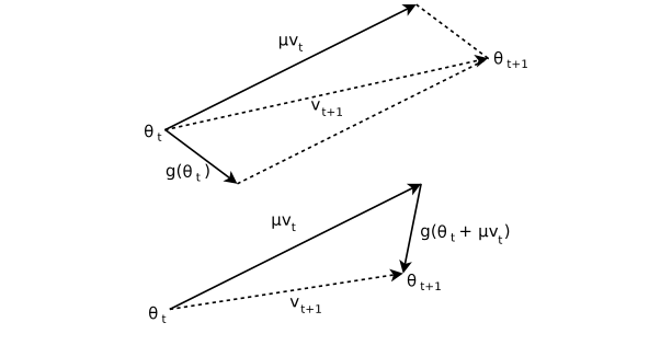
Nesterov acceleration technology was proposed by the great god Yurii Nesterov in 1983. It is very similar to the classic Momentum method used in deep learning. The difference from the momentum method is that the two use different points of gradient and momentum. The method uses the gradient of the previous iteration point, while the Nesterov method uses the gradient from the previous iteration point to one step forward. The specific comparison is as follows.
Momentum method:
Nesterov method:
The comparison shows that the Nesterov method and the momentum method are almost the same, but the gradient is slightly different. The following figure can more intuitively see the difference between the two.
Yuri Nestrov is a Russian mathematician and an internationally recognized expert in convex optimization, especially in efficient algorithm development and numerical optimization analysis. He is now a professor at the University of Rwanda.
The pseudo code of the FISTA algorithm is shown in the original text, and the matlab code is as follows:
function [x_2,error] = cs_fista(y,A,lambda,epsilon,itermax)
% Fast Iterative Soft Thresholding Algorithm(FISTA)
% Version: 1.0 written by yfzhang @2019-12-8
% Reference: Beck, Amir, and Marc Teboulle. "A fast iterative
% shrinkage-thresholding algorithm for linear inverse problems."
% SIAM journal on imaging sciences 2.1 (2009): 183-202.

% Inputs:
% y         - measurement vector
% A         - measurement matrix
% lambda    - denoiser parameter in the noisy case
% epsilon   - error threshold
% inter_max - maximum number of amp iterations
%
% Outputs:
% x_hat     - the last estimate
% error     - reconstruction error

if nargin < 5
    itermax = 10000 ;
end
if nargin < 4
    epsilon = 1e-4 ;
end
if nargin < 3
    lambda = 2e-5 ;
end

N = size(A,2);
error = [] ;

x_0 = zeros(N,1);
x_1 = zeros(N,1);
t_0 = 1 ;

for i = 1:itermax
    t_1 = (1+sqrt(1+4*t_0^2))/2 ;
    % g_1 = A'*(y-A*x_1);
    alpha =1;
    % alpha = (g_1'*g_1)/((A*g_1)'*(A*g_1)) ;
    z_2 = x_1 + ((t_0-1)/(t_1))*(x_1 - x_0) ;
    z_2 = z_2+A'*(y-A*z_2);
    x_2 = sign(z_2).*max(abs(z_2)-alpha*lambda,0) ;
    error(i,1) = norm(x_2 - x_1)/norm(x_2) ;
    error(i,2) = norm(y-A*x_2) ;
    if error(i,1) < epsilon || error(i,2) < epsilon
        break;
    else
        x_0 = x_1 ;
        x_1 = x_2 ;
        t_0 = t_1 ;
    end
end
4. Simulation experiment
In order to verify the performance of the ISTA algorithm and the FISTA algorithm, a one-dimensional random Gaussian signal is used as an experiment here. The test procedure is as follows:
% One-dimensional random Gaussian signal test script for CS reconstruction
% algorithm
% Version: 1.0 written by yfzhang @2019-12-8
clear
clc
N = 1024 ;
M = 512 ;
K = 10 ;
x = zeros(N,1);
T = 5*randn(K,1);
index_k = randperm(N);
x(index_k(1:K)) = T;

A = randn(M,N);
A=sqrt(1/M)*A;
A = orth(A')';
% sigma = 1e-4 ;
% e = sigma*randn(M,1);
y = A * x ;% + e ;

[x_rec1,error1] = cs_fista(y,A,5e-3,1e-4,5e3) ;
[x_rec2,error2] = cs_ista(y,A,5e-3,1e-4,5e3) ;

figure (1)
plot(error1(:,2),'r-');
hold on
plot(error2(:,2),'b-');
The simulation result diagram is as follows:
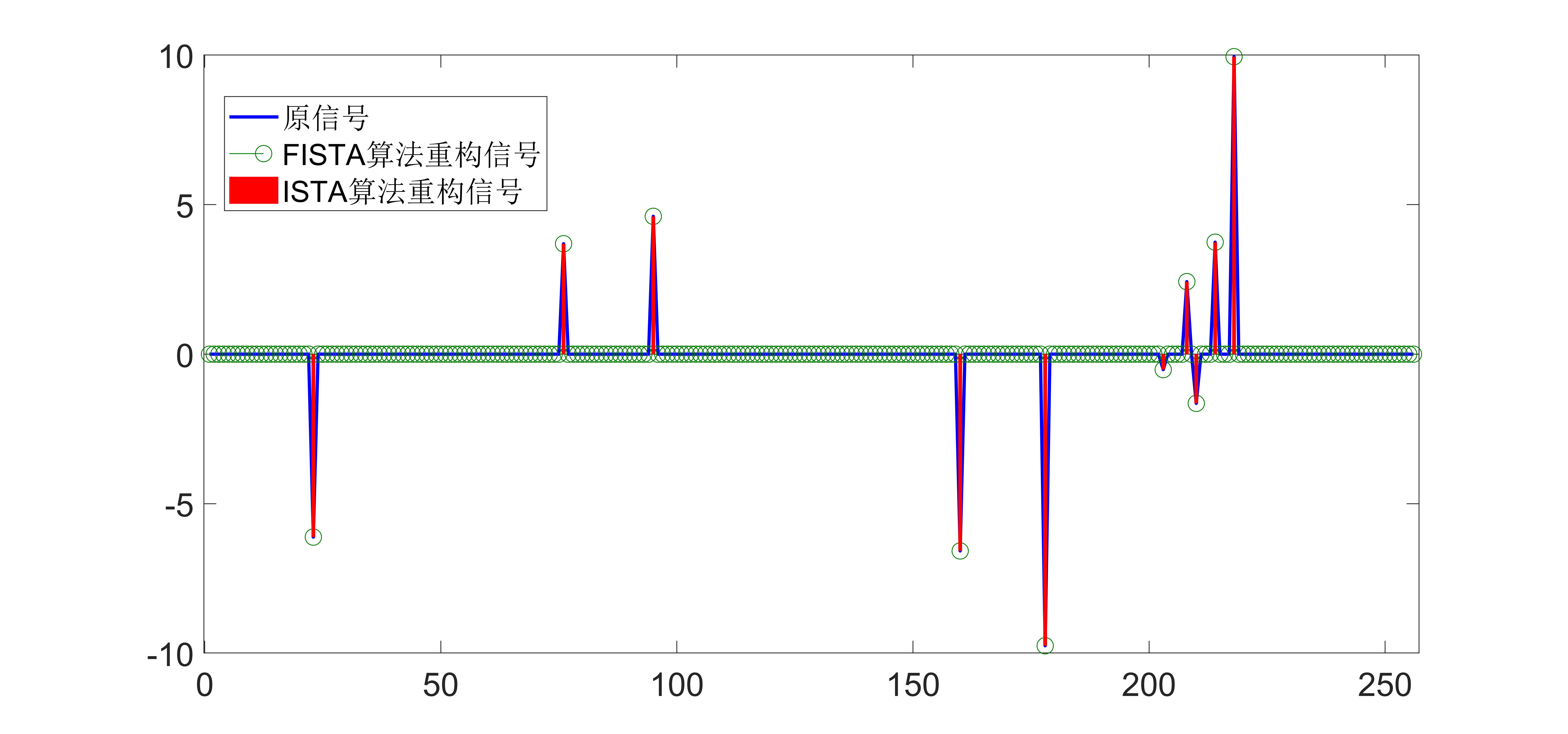
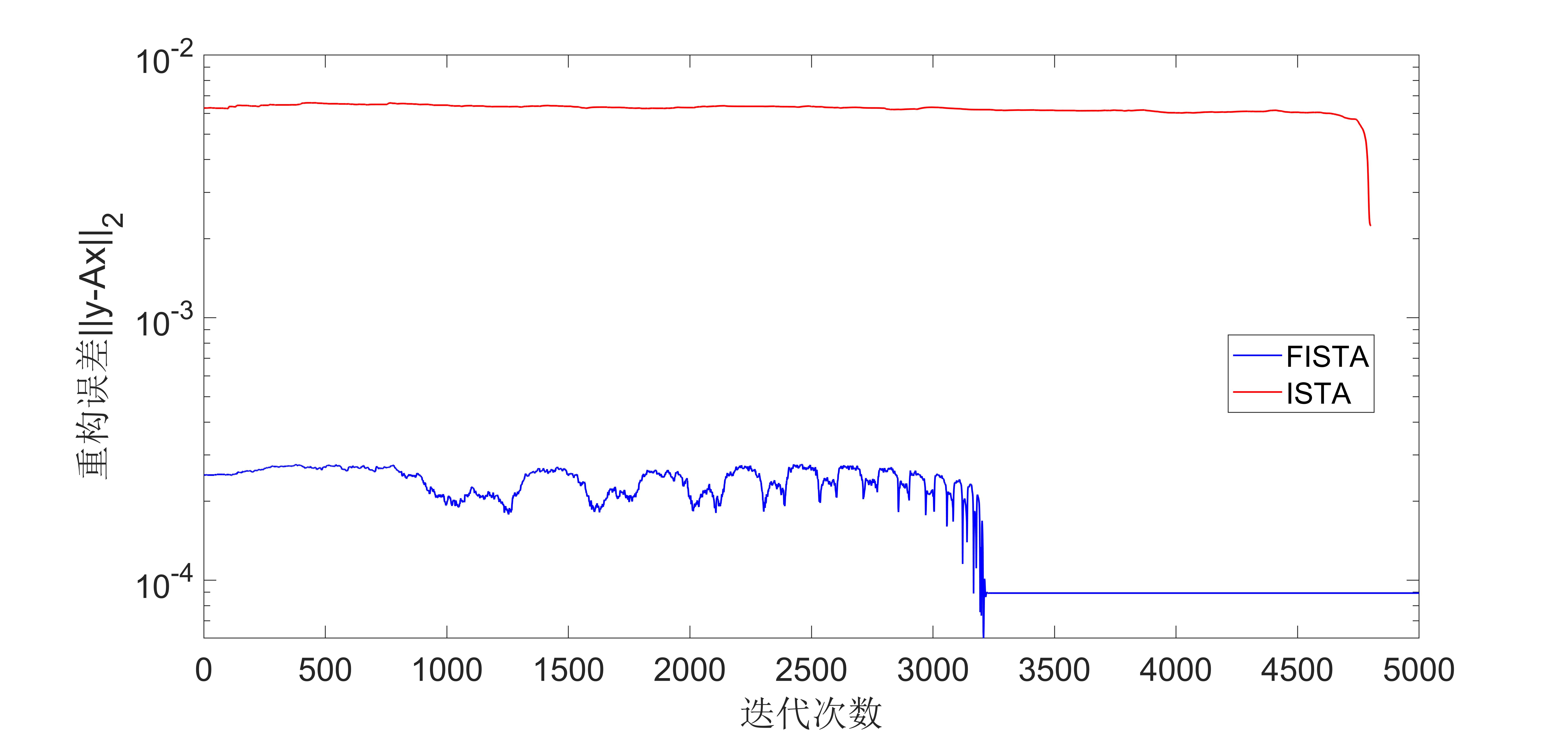
It can be seen from the experimental results that the convergence speed of the FIST algorithm is much faster than that of the ISTA algorithm.
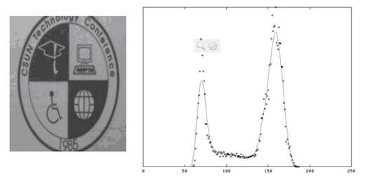
By the way, paste the experimental picture in the original text, which is about image denoising:


The figure shows the number of iterations and the denoising effect. The left is the FISTA algorithm, and the right is the ISTA algorithm. It is obvious that the FISTA algorithm is faster in denoising.
5. Discussion
Iterative Shrinkage Thresholding cannot actually be called an algorithm, but a kind of algorithm. The ISTA algorithm and FISTA and ISTA's improved algorithms such as the TWISTA algorithm all use soft threshold operations. Norm regularization problem (LASSO), and some algorithms use hard threshold operations. This type of algorithm is called iterative hard thresholding algorithm (Iterative Hard Thresholding). The problem that this type of algorithm solves is The problem of minimizing constraints is a non-convex optimization problem. Later, I have the opportunity to summarize the iterative hard threshold algorithm.
references
[1] Beck, Amir, and Marc Teboulle. “A fast iterative shrinkage-thresholding algorithm for linear inverse problems.” SIAM journal on imaging sciences 2.1 (2009): 183-202.
[2] Yurii E Nesterov., Dokl, akad. nauk Sssr. " A method for solving the convex programming problem with convergence rate O (1/k^ 2)" 1983.
For more exciting content, please follow the WeChat public account "Optimization and algorithm”

Intelligent Recommendation

ISTA algorithm
ISTA algorithm Article catalog ISTA algorithm 1 Introduction 2, iterative shrinkage threshold algorithm (ISTA) 1 Introduction For a basic linear inverse problem: y = A x + w \mathbf{y}=\mathbf{A}\math...
Research on Sophisticated Wavelet Soft Threshold Based on VMD
Research on Sophisticated Wavelet Soft Threshold Based on VMD Summary First, signal simulation Second, VMD noise reduction Second, VMD + wavelet soft threshold noise reduction to sum up Summary In thi...
Adaptive Threshold Algorithm
The maximum interclass variance method was proposed by the Japanese scholar Otsu in 1979. It is an adaptive threshold determination method, also known as Otsu. Law, referred to as OTSU. It divides the...
Adaptive threshold binarization algorithm
I. Introduction When a pair of black and white paper is photographed with a camera, the image obtained by the camera is not a true black and white image. Thi...
More Recommendation

Halcon algorithm and dynamic threshold
Picture path Link: https://pan.baidu.com/s/1ebcwmeq2nrwee8kWM0PH7Q Extract code: dtuj...
Adaptive Threshold Algorithm for OpenCV Local Threshold Segmentation
Foreword: When the illumination in the picture is uneven, the gray value of the image will be uneven. If we use the global threshold to share the same value for all pixel values, we can't get the idea...
Simple vision algorithm rewrite--threshold threshold
Simple vision algorithm rewrite--threshold threshold opencv is troublesome and the operating efficiency is too painful. Gradual split optimization...
R329-OPENCV threshold segmentation algorithm-adaptive threshold
R329-OPENCV threshold segmentation algorithm-adaptive threshold In the case of uneven lighting or uneven distribution of grayscale, if the global threshold is divided, the segmentation effect is often...
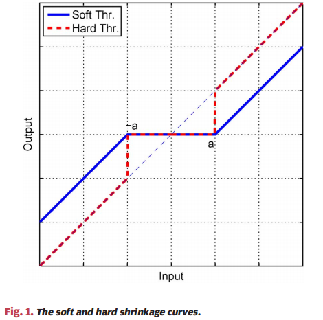
The difference between hard threshold function (Hard Thresholding) and soft threshold function (Soft Thresholding)
Once understood, it's actually extremely simple Commonly used soft threshold function is to solve the effect caused by hard threshold function "one size fits all" (modulo less than 3sigma wa...