Transformer of time series forecasting method
Recently I plan to share some time series forecasting methods based on machine learning. This is the third article.
Introduced earlierDeepAR with DeepState They are all based on RNN models. RNN is a classic method of sequence modeling. It obtains the global information of the sequence through recursion at the cost of not being able to be parallelized. CNN can also be used to model sequences, but because convolution captures local information, CNN models often need to stack many layers to get a larger receptive field. In the follow-up, I may ~~ (meaning not necessarily)~~ introduce the time series prediction method based on CNN. A masterpiece published by Google in 2017Attention Is All You Need It provides another way of thinking for sequence modeling, that is, relying solely on the Attention Mechanism to obtain global information in one step. Google calls this model Transformer. Transformer has achieved good results in fields such as natural language processing and image processing. The structure of Transformer is shown in the figure below (incorrect

This time I will introduce an article on NIPS 2019Enhancing the Locality and Breaking the Memory Bottleneck of Transformer on Time Series Forecasting, This article applies the Transformer model to time series forecasting1, And put forward some improvement directions.
We first introduce the attention mechanism, then briefly introduce the model, and finally give a demo.
Attention
According to Google’s plan, Attention is defined as
where
,
,
. From the dimension information of the matrix, it can be considered that Attention puts a
the sequence of
Code into one
New sequence. Remember
,
,
,can be seen
with
There is a one-to-one correspondence. Just look
For each vector in, there are
where
Is the normalization factor of the softmax function. It can be seen from the above formula that each
Are coded into
Weighted sum of
The weight depends on
versus
The inner product (dot multiplication) of. Scaling factor
Play a certain regulatory role to avoid the small gradient of softmax when the inner product is large. The attention mechanism under this definition is called Scaled Dot-Product Attention.
On the basis of Attention, Google also proposed Multi-Head Attention, which is defined as follows
where
,
. To put it simply,
、
with
Map to different representation spaces through linear transformation, and then calculate Attention; repeat
Times, take the
The results of Attention are spliced together, and finally one is output
the sequence of.
In Transformer, most of the Attentions are Self Attention ("self-attention" or "internal attention"), which means doing Attention within a sequence, that is . More precisely, it is Multi-Head Self Attention, which is . Self Attention can be understood as looking for sequence Links between different locations inside.
Model
What I said before is basically the content of the Google Transformer article, now we return to the article on time series prediction. To avoid confusion, we use Time Series Transformer to refer to the latter2。
Let’s review what we introduced earlierDeepAR Model: Assume the target value for each time step Obey probability distribution ; First use the LSTM unit to calculate the hidden state of the current time step , And then calculate the parameters of the probability distribution , And finally by maximizing the log likelihood To learn network parameters. The network structure of Time Series Transformer is similar to DeepAR, except that the LSTM layer is replaced with a Multi-Head Self Attention layer, which eliminates the need for recursion, but calculates all time steps at once. . As shown below3:
It should be noted that when forecasting the current time step, only the input up to the current time step can be used. Therefore, when calculating Attention, a Mask needs to be added, and the matrix The upper triangle element of is set to 。
On this basis, the article made two improvements to the model.
The first improvement is called Enhancing the locality of Transformer, which literally means to enhance the locality of Transformer. There are usually some abnormal points in the time series. Whether an observation should be regarded as an abnormality depends to a large extent on its context. And Multi-Head Self Attention
When calculating the relationship between different positions within the sequence, the local environment of each position is not considered, which makes the prediction susceptible to interference by outliers. At the beginning of the blog we already mentioned that convolution operations can be used to capture local information. If calculating
with
When using convolution instead of linear transformation, local information can be introduced in Self Attention. Note that since the current time step cannot use future information, causal convolution is used here.When introducing CNN-based timing prediction later, causal convolution will also play an important role.
The second improvement is called Breaking the memory bottleneck of Transformer. Assume that the sequence length is
, The calculation amount of Self Attention is
. In time series forecasting, long-range dependencies are often considered. In this case, memory usage will be considerable. In response to this problem, the article proposes the LogSparse Self Attention structure to reduce the amount of calculation to
,As shown below.
Code
By convention, here is a simple demo based on TensorFlow. It should be noted that this demo does not implement LogSparse Self Attention.
The Attention layer and Transformer model are defined as follows:
import tensorflow as tf

class Attention(tf.keras.layers.Layer):
    """
    Multi-Head Convolutional Self Attention Layer
    """
    def __init__(self, dk, dv, num_heads, filter_size):
        super().__init__()
        self.dk = dk
        self.dv = dv
        self.num_heads = num_heads

        self.conv_q = tf.keras.layers.Conv1D(dk * num_heads, filter_size, padding='causal')
        self.conv_k = tf.keras.layers.Conv1D(dk * num_heads, filter_size, padding='causal')
        self.dense_v = tf.keras.layers.Dense(dv * num_heads)
        self.dense1 = tf.keras.layers.Dense(dv, activation='relu')
        self.dense2 = tf.keras.layers.Dense(dv)

    def split_heads(self, x, batch_size, dim):
        x = tf.reshape(x, (batch_size, -1, self.num_heads, dim))
        return tf.transpose(x, perm=[0, 2, 1, 3])

    def call(self, inputs):
        batch_size, time_steps, _ = tf.shape(inputs)

        q = self.conv_q(inputs)
        k = self.conv_k(inputs)
        v = self.dense_v(inputs)

        q = self.split_heads(q, batch_size, self.dk)
        k = self.split_heads(k, batch_size, self.dk)
        v = self.split_heads(v, batch_size, self.dv)

        mask = 1 - tf.linalg.band_part(tf.ones((batch_size, self.num_heads, time_steps, time_steps)), -1, 0)

        dk = tf.cast(self.dk, tf.float32)

        score = tf.nn.softmax(tf.matmul(q, k, transpose_b=True)/tf.math.sqrt(dk) + mask * -1e9)

        outputs = tf.matmul(score, v)

        outputs = tf.transpose(outputs, perm=[0, 2, 1, 3])
        outputs = tf.reshape(outputs, (batch_size, time_steps, -1))

        outputs = self.dense1(outputs)
        outputs = self.dense2(outputs)

        return outputs

class Transformer(tf.keras.models.Model):
    """
    Time Series Transformer Model
    """
    def __init__(self, dk, dv, num_heads, filter_size):
        super().__init__()
        # Note that multiple Attentions are used in the article. For simplicity, this demo uses only one layer
        self.attention = Attention(dk, dv, num_heads, filter_size)
        self.dense_mu = tf.keras.layers.Dense(1)
        self.dense_sigma = tf.keras.layers.Dense(1, activation='softplus')

    def call(self, inputs):
        outputs = self.attention(inputs)
        mu = self.dense_mu(outputs)
        sigma = self.dense_sigma(outputs)

        return [mu, sigma]
For the loss function and training part, please refer to our introductionDeepAR The demo given at the time.
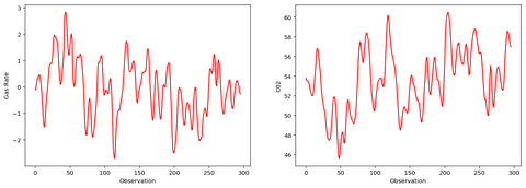
To verify the code, we randomly generate a time series with a period. The figure below shows part of the data points of this sequence.
The difference with DeepAR is that because the Attention structure does not capture the sequence of the sequence well, we added the relative position as a feature.
After training, it is used for prediction, and the effect is shown in the figure below. The shaded part represents the interval from 0.05 quantile to 0.95 quantile.
Compared with DeepAR
- In a sense, the network structures of the two are very similar, and they are all learning the parameters of the probability distribution.
- The Attention structure itself cannot well capture the sequence of the sequence. Of course, this is not a big problem, because usually timing prediction tasks will have time characteristics, and there is no need to add additional positional coding as in natural language processing.
- The experimental results given in this article show that Time Series Transformer has more advantages than DeepAR in capturing long-range dependencies.
- Time Series Transformer can be calculated in parallel during training, which is better than DeepAR. However, because it uses the same autoregressive structure as DeepAR, it cannot be parallelized when predicting. Not only that, when DeepAR predicts a single time step, it only needs to use the current input and the hidden state of the previous step's output; while the Transformer needs to calculate the global Attention. Therefore, when predicting, the calculation efficiency of Transformer is likely to be inferior to DeepAR.
Strictly speaking, this article is not using Transformer. Google's Transformer is an Encoder-Decoder structure, and the network structure used in this article actually replaces the LSTM layer in DeepAR with a Multi-Head Self Attention layer. This structure is actually a (incomplete) Transformer Decoder part. But, whatever...︎
There is no such saying in the original text.︎
This picture was drawn by myself, the original text is not available.︎
Intelligent Recommendation

Stationary time series forecasting
The so-called prediction is to use the known sample value of the sequence to estimate the value of the sequence at a certain time in the future. At present, the most commonly used prediction method fo...
Time series forecasting-ARIMA
Reference 1 https://pyflux.readthedocs.io/en/latest/arima.html#example Reference 2 Multivariate sequence analysis ARIMAX(p,I,q) Uchiha belt soil Nothing to mess around 4 people agreed with the ...
keras time series forecasting
keras time series forecasting num represents the number of bicycles, weekday represents the day of the week, and hour represents the hour. A total of 45949 pieces of data are arranged in the order of ...

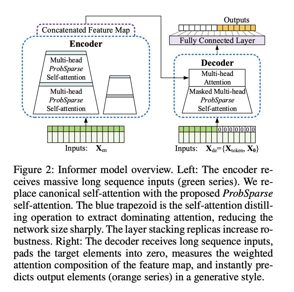
Informer: Beyond Effectient Transformer for Long Sequence Time-Series Forecasting Papers Interpretation
Informer:Beyond Efficient Transformer for Long Sequence Time-Series Forecasting 1. Introduction 2. Preliminary 3. Methodology 3.1 Efficient self-focus mechanism 3.2 Encoder: Allows longer sequential i...
2021.06.16 Group Report Informer: Beyond Efficient Transformer for Long Sequence Time-Series Forecasting
2021.06.16 Group Report Informer: Beyond Efficient Transformer for Long Sequence Time-Series Forecasting Related background 2. Main problems 2.1 ProbSparse Self-attention 2.2 Self-attention Distilling...
More Recommendation
[Paper Reading] Informer: Beyond Efficient Transformer for Long Sequence Time-Series Forecasting
[Paper Reading] Informer: Beyond Efficient Transformer for Long Sequence Time-Series Forecasting Original: https://arxiv.org/abs/2012.07436 code (pytorch implementation): https://github.com/zhouhaoyi/...
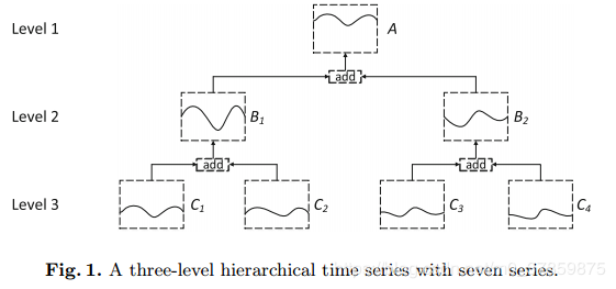
Multi-task Learning Method for Hierarchical Time Series Forecasting
Multi-task Learning Method for Hierarchical Time Series Forecasting motivation Main contribution Formal definition Two models MHFM(multi-task hierarchical forecasting model) DMHFM(dirty multi-task hie...
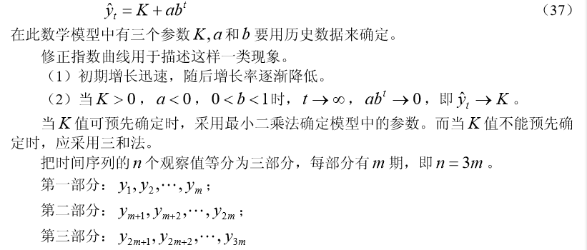
Time series model (5): Trend extrapolation forecasting method
Other blog posts in time series: Time series model (1): model overview Time series model (2): moving average method Time series model (3): Exponential smoothing method Time series model (4): Differenc...

spss time series forecasting sales
First, there is the concept of time series of a general understanding that the same variable to predict the future value of a variable based on past observations, is to predict the future based on exi...
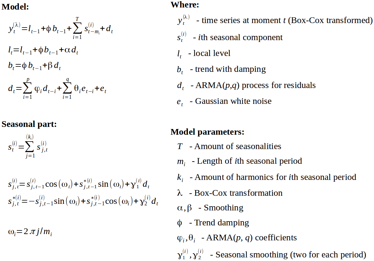
Time series forecasting model TBATS
1. Introduction to TBATS Name origin: Trigonometric seasonality, Box-Cox transformation, ARMA errors, Trend and Seasonal components. The model uses seasonal features, Box-Cox transformation, ARMA erro...