PCA principle and python implementation
Data dimensionality reduction
In machine learning, data is usually input to the model in the form of vectors for training. As we all know, when the data has more features and the vector has a larger dimension, the process of processing the data and the process of training the model will consume greatly the memory space of the system and increase the training of the model. Time cost, and even dimensionality disaster (Curse of Dimensionality: usually refers to a phenomenon in which the amount of calculation increases exponentially as the dimensionality increases in problems involving the calculation of vectors). Therefore, to reduce the dimensionality of the data, it is particularly important to use low-dimensional vectors to represent the original high-dimensional vectors. Common dimensionality reduction methods are: principal component analysis, linear discriminant analysis, isometric mapping, local linear embedding, Laplacian feature mapping, local retention projection, etc.
Among them, principal component analysis is the most classic dimensionality reduction method. This article will make a systematic summary of the recent review of PCA dimensionality reduction.
PCA dimensionality reduction
As the name suggests, PCA dimensionality reduction is to find the principal components of the data, and then use these principal components to represent the original data. As shown in the figure below, all data samples are represented by the two features of X1 and X2.
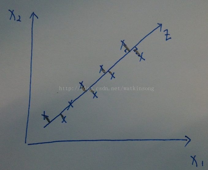
It can be seen that almost all samples are distributed on a straight line, so this straight line can be used as a coordinate axis, and all data can be approximated by this coordinate axis. Therefore, the feature is reduced from two dimensions to one dimension.
In the field of signal processing, it is generally considered that the signal has a large variance and the noise has a small variance. The ratio of the variance of the signal to the variance of the noise is called the signal-to-noise ratio. The higher the signal-to-noise ratio, the higher the quality of the data, and vice versa. As can be seen from the above figure, the projection points of the data on the axis where the principal components are located are the most scattered, and the projection variance is also the largest. Therefore, it can be seen that the PCA dimensionality reduction process is to find an axis W that maximizes the projection variance of the original data on this axis.
For a given set of data, {v1,v2,v3,…,vn}, decentralized, expressed as {x1,x2,x3,…,xn} = {v1 -u, v2-u, v3-u, …, vn-u}, where u=
. (As for why centralization is required, I will not show it here for the time being, it will be clear later). vector
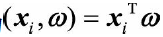
On axis
The projected coordinates on can be expressed as:
The goal of PCA is to find such a
, Making
in
The projection variance on the projected coordinates is maximized. The average value of the projected coordinates can be expressed as:
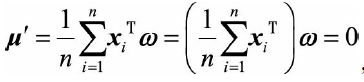
Do you understand the purpose of centralized processing of raw data? In fact, the mean value of the projection coordinates of the data is 0, which is convenient for calculating the maximum projection variance later. The projection variance can be expressed as:
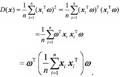
The middle part of the above formula
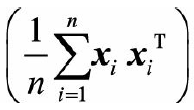
is the covariance matrix of the data sample, using Said. In addition, due to
Is a unit vector, so
Said. In addition, due to
Is a unit vector, so 。
。
So we ask to solve a maximization problem, which can be expressed as:
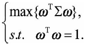
introduces Lagrangian multipliers, and
Take the derivative so that it is zero, you can get
Obviously,
Is the eigenvalue of the covariance matrix,
Eigenvalue
The corresponding feature vector. The projection variance can be expressed as:
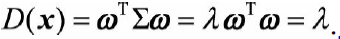
The projection variance is equal to the eigenvalue of the covariance matrix. The largest projection variance is only required for the largest eigenvalue of the covariance matrix, and the best projection direction corresponds to the eigenvector corresponding to the largest eigenvalue. The secondary projection direction corresponds to the eigenvector corresponding to the second largest eigenvalue. By analogy, a K-dimensional space composed of eigenvectors corresponding to the first K largest eigenvalues of the covariance matrix can be obtained to represent the original data, that is, the n-dimensionality of the original data is reduced to K-dimensionality.
The PCA solution process can be summarized as follows:
(1) Centralize the original data (to facilitate the calculation of projection variance in the later stage)
(2) Find the covariance matrix of the sample after centralization
(3) Solve the eigenvalues of the covariance matrix and the corresponding eigenvectors
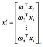
(4) Select the eigenvectors corresponding to the first d largest eigenvalues of the covariance matrix to construct a d-dimensional space, and map the n-dimensional sample to the d-dimensional through the following mapping:
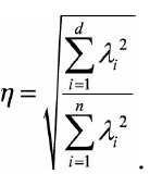
The proportion of information after dimensionality reduction is:
The above is the process of analyzing PCA dimensionality reduction theory from the perspective of maximum variance theory. In addition, PCA dimensionality reduction can also be explained from the perspective of the minimum regression error to construct the loss function. The specific process is detailed at https://www.cnblogs.com/sowhat4999/p/5824880.html
import numpy as np
class PCA:
def __init__(self, X):
self.X = X
self.mean = None
self.feature = None
def transform_data(self, n_components = 1):
n_samples, n_features = self.X.shape #Number of samples and the number of features in each sample
self.mean = np.array([np.mean(self.X[:, i]) for i in range(n_features)]) #average of each feature
norm_X = self.X-self.mean #Centralize the original data
scatter_X = np.dot(norm_X.T, norm_X) #The covariance matrix of the data sample
eig_val, eig_vec = np.linalg.eig(scatter_X) #Solve the eigenvalues of the covariance matrix and the eigenvector corresponding to each eigenvalue
eig_pairs = [(np.abs(eig_val[i]), eig_vec[:, i]) for i in range(len(eig_val))]
eig_pairs.sort(reverse = True) #Sort the feature values in order from largest to smallest
self.feature = np.array([ele[1] for ele in eig_pairs[:n_components]) #take the first n_components feature vectors
new_data = np.dot(norm_X, self.feature.T) #Data after dimensionality reduction
return new_data
def inverse_transform(self, new_data):
return np.dot(new_data, self.feature) + self.mean
def load_dataset(filepath):
return np.loadtxt(filepath, dtype = np.float)
if __name__ == "__main__":
X = load_datatxt('D:/The heart of the machine/current learning/PCA/pca-master/data/testPCA4.txt') #import data
myPCA = PCA(X = X)
new_data = myPCA.transform(n_components = 1)
origin_data = myPCA.inverse_transform(new_data = new_data)
print("After reducing the data to {}, the variance ratio before and after the data is {}".format(new_data.shape[1], np.var(new_data)/np.var(origin_data)
Of course, if we don’t want to make our own wheels, we can also directly call the PCA API.
from sklearn.decomposition import PCA
pca = PCA(n_components  = 1)
X = load_datatxt('D:/The heart of the machine/current learning/PCA/pca-master/data/testPCA4.txt')
new_data = pca.fit_transform(X)
origin_data = pca.inverse_data(new_data)
 print("After reducing the data to {}, the variance ratio before and after the data is {}".format(new_data.shape[1], np.var(new_data)/np.var(origin_data)
The above is my humble opinion on the most classic PCA algorithm among the dimensionality reduction algorithms. I hope that I can criticize and correct the shortcomings!
Intelligent Recommendation
Python implementation PCA
achieve Based on Python with a powerful sklearn library, it is very suitable for machine learning, so here python is used as an example. First, the training set has 6 sets of data, each set has 4 feat...
PCA - Python implementation
Article directory PCA principle Code implementation (python) PCA principle Pca mainly achieves the purpose of dimensionality reduction by calculating the eigenvectors of the matrix and using the matri...

PCA-Python implementation (2)
Article Directory 1. Introduction of simple concepts 1.1 The difference between numpy's .std() and pandas' .std() functions 1.2 np.linalg.svd() 1.3 Application of PCA 2. PCA calculation process 2.1 Fe...
PCA python implementation
PCA (Principal Component Analysis) is a method to achieve dimensionality reduction, and its principles involve variance, covariance, SVD, and so on. Derivation process link: The details of the impleme...

More Recommendation
PCA-python implementation
One, pca implementation steps 1. Zero averaging. Find the average of each column of the matrix, and then subtract this average from all the numbers in the column. 2. Find the covariance matrix. Both p...
PCA principle code implementation-examples
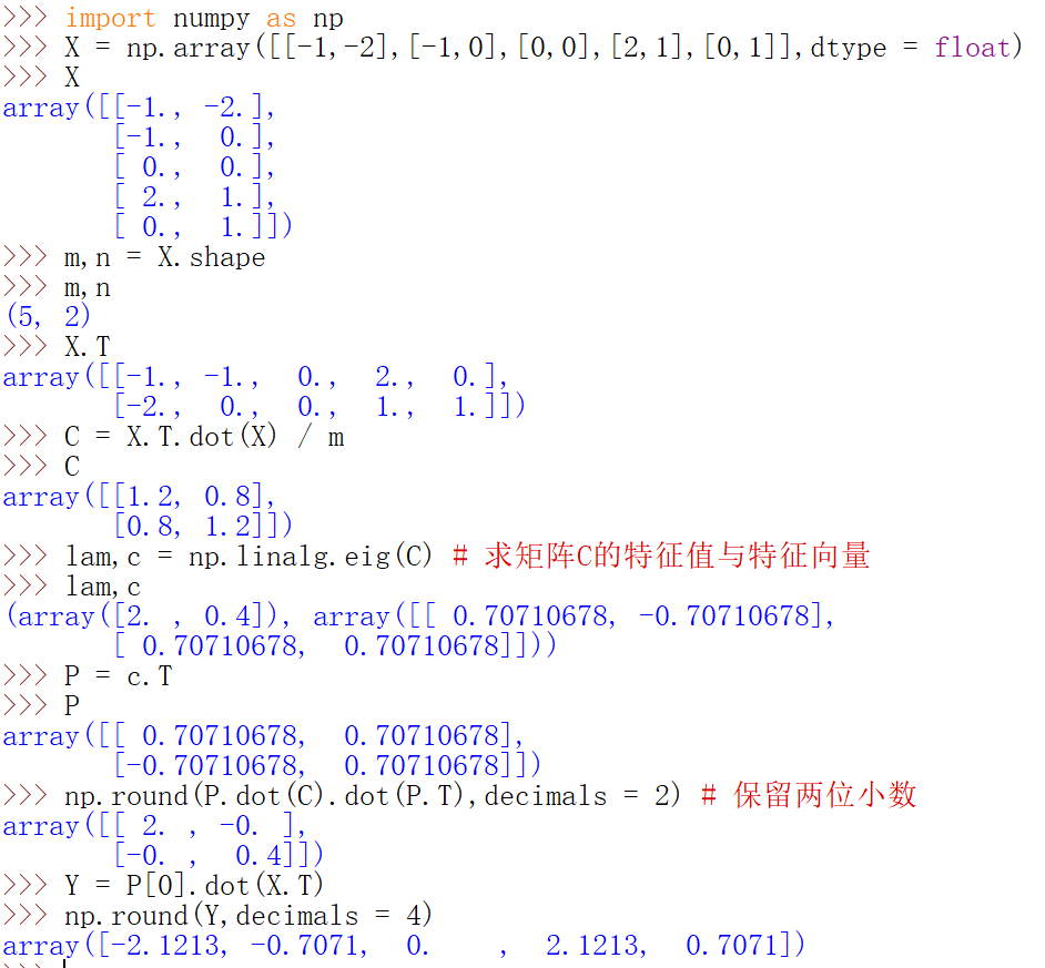
Assumption: [ − 1 − 1 0 2 0 − 2 0 0 1 1 ] \begin{bmatrix} -1 & -1 & 0 & 2 & 0 \\ -2 & 0 & 0 & 1 & 1 \end{bmatrix} [−1−2−10002101...
Principle of PCA algorithm and C++ implementation
PCA principal component analysis is a common feature reduction algorithm in pattern recognition. The general steps can be divided into the following parts: (1) Normalization of the original feature ma...
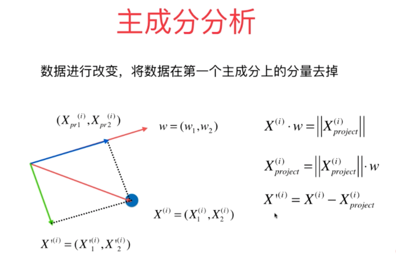
Python realizes the principle of PCA algorithm
Data principal component analysis process of PCA principal component analysis method and implementation of python principle 1. For principal component analysis,After the first principal component is o...