Read the background knowledge points required for this article: matrix to guide, throw a programming knowledge

I. Introduction

Previously, the two dual classification algorithms -perception algorithm and pocket algorithm are introduced. These algorithms are solved with classification problems, but in reality, more, such as predicting housing prices in a certain area, how much banks should bank give someone a certain amount of people to someone to give someone a certain amount of someone to a certain amount Credit cards, how many stocks should be traded today, etc. The last specific numerical result is a problem. This type of problem is called a regression problem in machine learning.

The regression analysis is a method of studying multiple groups of variables in statistics. It is also widely used in machine learning. The following introduces one of the algorithm models-Linear regression¹（Linear Regression）

2. Model introduction

Before introducing the model, let's take a look at an example. Assuming that some places have counted the income of people in different working years (analog data), as shown in the table below:

Working life	Average monthly salary
1 year	1598 yuan
2 years	3898 yuan
3 years	6220 yuan
4 years	7799 yuan
5 years	10510 yuan

From the data in the above table, you can draw an image of the average monthly income every other year:

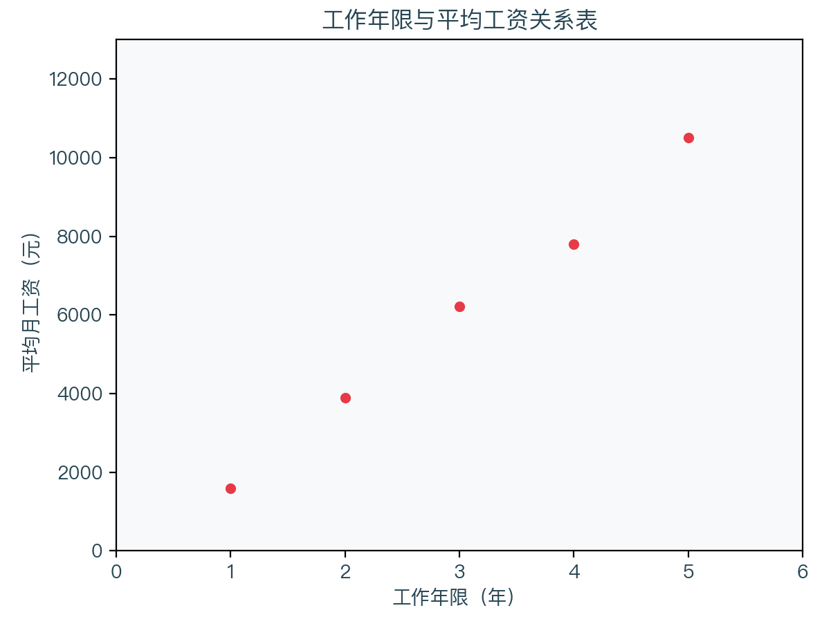
From the figure above, it can be seen that these points seem to be on a straight line or near them. We can judge that the local average monthly income and working years can seem to have a certain linear relationship based on intuition. We can predict the average monthly income of people with a 6 -year salary period. The process of finding such a straight line is called a linear regression analysis.

Definition: Given some random sample points {x1, y1}, {x2, y2}, ..., find a ultra -flat plane (a straight line when a single variable is a straight line, two variables is a plane) to fit these sample points. The linear equation is as follows:

(1) General form of ultra -plane function equation

(2) Like the perception of algorithm, think B as the zero W, and abbreviate the ultra -plane function equation into the form of two vectors W and X point accumulation.

y = b + w 1 x 1 + w 2 x 2 + ⋯ + w M x M = w T x \begin{array}{rcc} y & =b+w_{1} x_{1}+w_{2} x_{2}+\cdots+w_{M} x_{M} \\ & =\quad w^{T} x \end{array} y​=b+w1​x1​+w2​x2​+⋯+wM​xM​=wTx​

Single variables are straight lines, two variables are plane, and multi -variables are ultra -flat planes

Third, algorithm steps

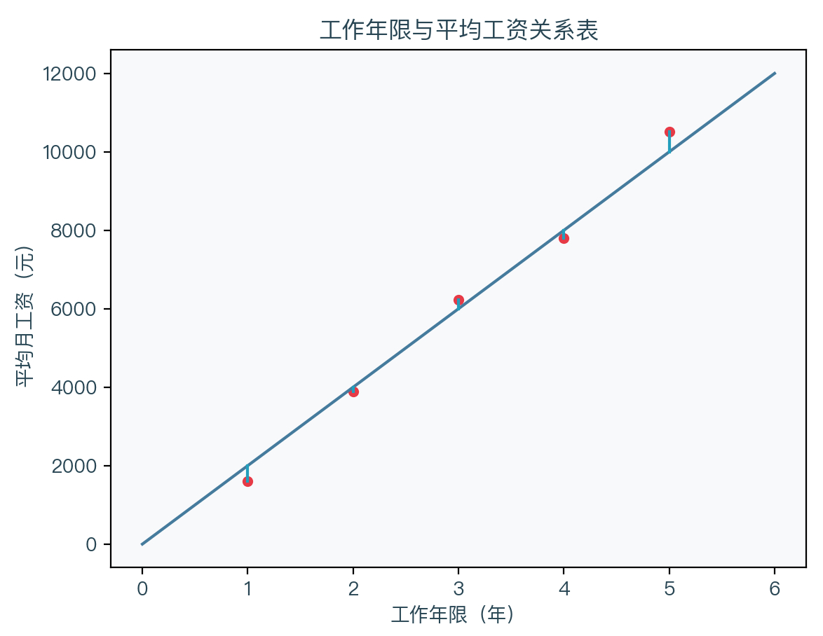
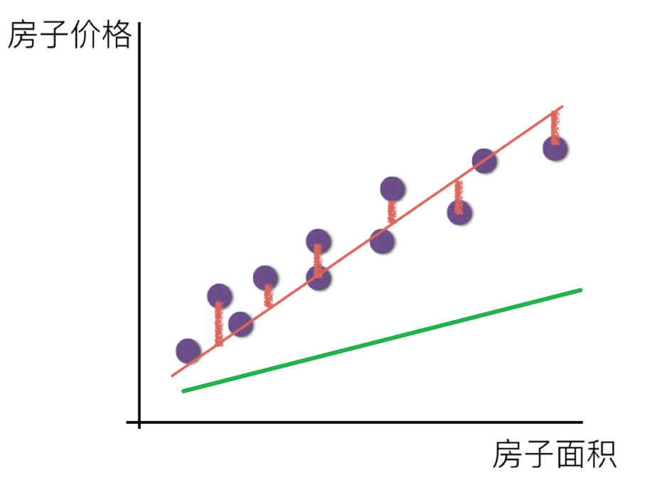
So how to find the best super plane from a bunch of sample points? In the example of the above and average monthly salary, it seems that many straight lines can be drawn to fit these points.

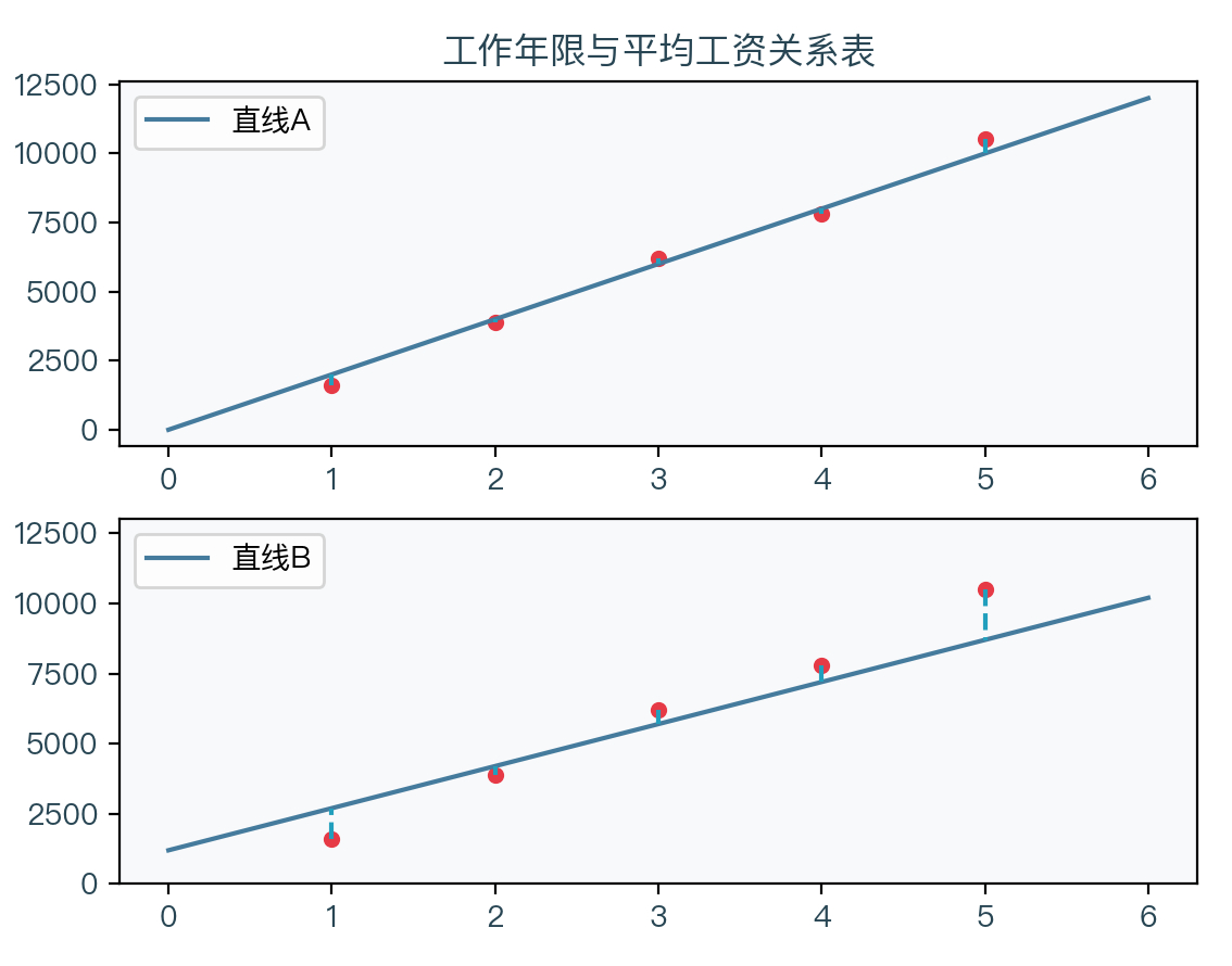
Just like the two straight lines above, which straight line is better on it? It should be seen through the dotted line in the figure. The distance between each sample point and the line B is relatively far A. The line A is obviously better than that of the straight line B, which means that the distance between the sample point and the straight line can be To judge the good or bad situation of fit.

Assuming that there are n sample points {x, y}, the self -variables of each sample point are m {x1, x2, ...}, then the sum of the distance between all sample points and this ultra -plane is to fit these sample points to fit these sample points The cost function, where W is the M -dimensional serial vector, X is also the M -dimensional column vector, Y is the real number:

Cost ⁡ ( w ) = ∑ i = 1 N ∣ w T x i − y i ∣ \operatorname{Cost}(w)=\sum_{i=1}^{N}\left|w^{T} x_{i}-y_{i}\right| Cost(w)=i=1∑N​∣∣​wTxi​−yi​∣∣​

Because there is an absolute value in the function, it is rewritten into a square form, which is called in geometry.Ouji miles distance²。

Cost ⁡ ( w ) = ∑ i = 1 N ( w T x i − y i ) 2 \operatorname{Cost}(w)=\sum_{i=1}^{N}\left(w^{T} x_{i}-y_{i}\right)^{2} Cost(w)=i=1∑N​(wTxi​−yi​)2

Interestingly, we only need to minimize the value of the cost function, that is, the time of the distance between the Ouji of all sample points to the ultra -plane is the smallest, and the corresponding W is the weight coefficient of this ultra -flat plane.

w = argmin ⁡ w ( ∑ i = 1 N ( w T x i − y i ) 2 ) w=\underset{w}{\operatorname{argmin}}\left(\sum_{i=1}^{N}\left(w^{T} x_{i}-y_{i}\right)^{2}\right) w=wargmin​(i=1∑N​(wTxi​−yi​)2)

[argmin](https://en.wikipedia.org/wiki/Arg_max#Arg_min)³ Function represents the variable at this time

The method of solving based on the minimization of the above function is called the minimum daily method. Because the cost function is aConvex function⁴According to the nature of the convex function, it can be seen that its local minimum value is the global minimum value. You can directly obtain the best analysis and solution of W.

w = ( X T X ) − 1 X T y w=\left(X^{T} X\right)^{-1} X^{T} y w=(XTX)−1XTy

X = [ x 1 T x 2 T ⋮ x N T ] = [ X 11 X 12 ⋯ X 1 M X 21 X 22 ⋯ X 2 M ⋮ ⋮ ⋱ ⋮ X N 1 X N 2 ⋯ X N M ] y = ( y 1 y 2 ⋮ y N ) X=\left[\begin{array}{c} x_{1}^{T} \\ x_{2}^{T} \\ \vdots \\ x_{N}^{T} \end{array}\right]=\left[\begin{array}{cccc} X_{11} & X_{12} & \cdots & X_{1 M} \\ X_{21} & X_{22} & \cdots & X_{2 M} \\ \vdots & \vdots & \ddots & \vdots \\ X_{N 1} & X_{N 2} & \cdots & X_{N M} \end{array}\right] \quad y=\left(\begin{array}{c} y_{1} \\ y_{2} \\ \vdots \\ y_{N} \end{array}\right) X=⎣⎢⎢⎢⎡​x1T​x2T​⋮xNT​​⎦⎥⎥⎥⎤​=⎣⎢⎢⎢⎡​X11​X21​⋮XN1​​X12​X22​⋮XN2​​⋯⋯⋱⋯​X1M​X2M​⋮XNM​​⎦⎥⎥⎥⎤​y=⎝⎜⎜⎜⎛​y1​y2​⋮yN​​⎠⎟⎟⎟⎞​

Fourth, proven

Linear regression cost function is a convex function

The convex function is a real value function F on the convex set C of a vector space, and for the two vectors X1 in the arbitrary set C in the convex set C, the x2 satisfies the following formula:

f ( x 1 + x 2 2 ) ≤ f ( x 1 ) + f ( x 2 ) 2 f\left(\frac{x_{1}+x_{2}}{2}\right) \leq \frac{f\left(x_{1}\right)+f\left(x_{2}\right)}{2} f(2x1​+x2​​)≤2f(x1​)+f(x2​)​

The left side of the inconsistency:

Cost ⁡ ( w 1 + w 2 2 ) = ∑ i = 1 N [ ( w 1 + w 2 2 ) T x i − y i ] 2 \operatorname{Cost}\left(\frac{w_{1}+w_{2}}{2}\right)=\sum_{i=1}^{N}\left[\left(\frac{w_{1}+w_{2}}{2}\right)^{T} x_{i}-y_{i}\right]^{2} Cost(2w1​+w2​​)=i=1∑N​[(2w1​+w2​​)Txi​−yi​]2

The right side of the way:

Cost ⁡ ( w 1 ) + Cost ⁡ ( w 2 ) 2 = ∑ i = 1 N ( w 1 T x i − y i ) 2 + ∑ i = 1 N ( w 2 T x i − y i ) 2 2 \frac{\operatorname{Cost}\left(w_{1}\right)+\operatorname{Cost}\left(w_{2}\right)}{2}=\frac{\sum_{i=1}^{N}\left(w_{1}^{T} x_{i}-y_{i}\right)^{2}+\sum_{i=1}^{N}\left(w_{2}^{T} x_{i}-y_{i}\right)^{2}}{2} 2Cost(w1​)+Cost(w2​)​=2∑i=1N​(w1T​xi​−yi​)2+∑i=1N​(w2T​xi​−yi​)2​

(1) Multiplying on the left side of the inequality

(2) Move 2 into the plus operation, write three items

(3) Open the square in 6 items

2 Cost ⁡ ( w 1 + w 2 2 ) = 2 ∑ i = 1 N [ ( w 1 + w 2 2 ) T x i − y i ] 2 ( 1 ) = ∑ i = 1 N 2 ( w 1 T x i 2 + w 2 T x i 2 − y i ) 2 ( 2 ) = ∑ i = 1 N ( w 1 T x i x i T w 1 2 + w 2 T x i x i T w 2 2 + w 1 T x i w 2 T x i − 2 w 1 T x i y i − 2 w 2 T x i y i + 2 y i 2 ) ( 3 ) \begin{aligned} 2 \operatorname{Cost}\left(\frac{w_{1}+w_{2}}{2}\right) &=2 \sum_{i=1}^{N}\left[\left(\frac{w_{1}+w_{2}}{2}\right)^{T} x_{i}-y_{i}\right]^{2} & (1) \\ &=\sum_{i=1}^{N} 2\left(\frac{w_{1}^{T} x_{i}}{2}+\frac{w_{2}^{T} x_{i}}{2}-y_{i}\right)^{2} & (2) \\ &=\sum_{i=1}^{N}\left(\frac{w_{1}^{T} x_{i} x_{i}^{T} w_{1}}{2}+\frac{w_{2}^{T} x_{i} x_{i}^{T} w_{2}}{2}+w_{1}^{T} x_{i} w_{2}^{T} x_{i}-2 w_{1}^{T} x_{i} y_{i}-2 w_{2}^{T} x_{i} y_{i}+2 y_{i}^{2}\right) & (3) \end{aligned} 2Cost(2w1​+w2​​)​=2i=1∑N​[(2w1​+w2​​)Txi​−yi​]2=i=1∑N​2(2w1T​xi​​+2w2T​xi​​−yi​)2=i=1∑N​(2w1T​xi​xiT​w1​​+2w2T​xi​xiT​w2​​+w1T​xi​w2T​xi​−2w1T​xi​yi​−2w2T​xi​yi​+2yi2​)​(1)(2)(3)​

(1) Multiply 2 on the right side

)

(3) Expand the square items in the bracket

(4) Move items to be consistent with the above

Cost ⁡ ( w 1 ) + Cost ⁡ ( w 2 ) = ∑ i = 1 N ( w 1 T x i − y i ) 2 + ∑ i = 1 N ( w 2 T x i − y i ) 2 ( 1 ) = ∑ i = 1 N [ ( w 1 T x i − y i ) 2 + ( w 2 T x i − y i ) 2 ] ( 2 ) = ∑ i = 1 N ( w 1 T x i x i T w 1 − 2 w 1 T x i y i 2 + y i 2 + w 2 T x i x i T w 2 − 2 w 2 T x i y i + y i 2 ) ( 3 ) = ∑ i = 1 N ( w 1 T x i x i T w 1 + w 2 T x i x i T w 2 − 2 w 1 T x i y i − 2 w 2 T x i y i + 2 y i 2 ) ( 4 ) \begin{aligned} \operatorname{Cost}\left(w_{1}\right)+\operatorname{Cost}\left(w_{2}\right) &=\sum_{i=1}^{N}\left(w_{1}^{T} x_{i}-y_{i}\right)^{2}+\sum_{i=1}^{N}\left(w_{2}^{T} x_{i}-y_{i}\right)^{2} & (1) \\ &=\sum_{i=1}^{N}\left[\left(w_{1}^{T} x_{i}-y_{i}\right)^{2}+\left(w_{2}^{T} x_{i}-y_{i}\right)^{2}\right] & (2)\\ &=\sum_{i=1}^{N}\left(w_{1}^{T} x_{i} x_{i}^{T} w_{1}-2 w_{1}^{T} x_{i} y_{i}^{2}+y_{i}^{2}+w_{2}^{T} x_{i} x_{i}^{T} w_{2}-2 w_{2}^{T} x_{i} y_{i}+y_{i}^{2}\right) & (3)\\ &=\sum_{i=1}^{N}\left(w_{1}^{T} x_{i} x_{i}^{T} w_{1}+w_{2}^{T} x_{i} x_{i}^{T} w_{2}-2 w_{1}^{T} x_{i} y_{i}-2 w_{2}^{T} x_{i} y_{i}+2 y_{i}^{2}\right) & (4) \end{aligned} Cost(w1​)+Cost(w2​)​=i=1∑N​(w1T​xi​−yi​)2+i=1∑N​(w2T​xi​−yi​)2=i=1∑N​[(w1T​xi​−yi​)2+(w2T​xi​−yi​)2]=i=1∑N​(w1T​xi​xiT​w1​−2w1T​xi​yi2​+yi2​+w2T​xi​xiT​w2​−2w2T​xi​yi​+yi2​)=i=1∑N​(w1T​xi​xiT​w1​+w2T​xi​xiT​w2​−2w1T​xi​yi​−2w2T​xi​yi​+2yi2​)​(1)(2)(3)(4)​

Skine the items on the right side of the non -equivalent formula to the left side of the inconsistent left, and remember the difference obtained as Δ. Now it is only necessary to prove that the difference between the two items is greater than equal to zero.

(1) Observe the results of the two items. The last 3 items are the same.

(2) Proposal one -half of them

(3) Observing the brackets will be found as a square form

Δ = ∑ i = 1 N ( w 1 T x i x i T w 1 2 + w 2 T x i x i T w 2 2 − w 1 T x i w 2 T x i ) ( 1 ) = 1 2 ∑ i = 1 N ( w 1 T x i x i T w 1 + w 2 T x i x i T w 2 − 2 w 1 T x i w 2 T x i ) ( 2 ) = 1 2 ∑ i = 1 N ( w 1 T x i − w 2 T x i ) 2 ( 3 ) \begin{aligned} \Delta &=\sum_{i=1}^{N}\left(\frac{w_{1}^{T} x_{i} x_{i}^{T} w_{1}}{2}+\frac{w_{2}^{T} x_{i} x_{i}^{T} w_{2}}{2}-w_{1}^{T} x_{i} w_{2}^{T} x_{i}\right) & (1) \\ &=\frac{1}{2} \sum_{i=1}^{N}\left(w_{1}^{T} x_{i} x_{i}^{T} w_{1}+w_{2}^{T} x_{i} x_{i}^{T} w_{2}-2 w_{1}^{T} x_{i} w_{2}^{T} x_{i}\right) & (2) \\ &=\frac{1}{2} \sum_{i=1}^{N}\left(w_{1}^{T} x_{i}-w_{2}^{T} x_{i}\right)^{2} & (3) \end{aligned} Δ​=i=1∑N​(2w1T​xi​xiT​w1​​+2w2T​xi​xiT​w2​​−w1T​xi​w2T​xi​)=21​i=1∑N​(w1T​xi​xiT​w1​+w2T​xi​xiT​w2​−2w1T​xi​w2T​xi​)=21​i=1∑N​(w1T​xi​−w2T​xi​)2​(1)(2)(3)​

The difference between the left side of the inconsistency on the right of the unlimal form is a square additional computing, and the final result within the real range must be greater than equal to zero, and the certificate is completed.

Analysis of linear regression cost function

(1) The cost function of linear regression

(2) It can be rewritten into the form of two N -dimensional vectors.

(3) Use A to indicate the first N -dimensional vector, the cost function is actually the conversion of the A vector by the A vector

Cost ⁡ ( w ) = ∑ i = 1 N ( w T x i − y i ) 2 ( 1 ) = ( w T x 1 − y 1 … w T x N − y N ) ( w T x 1 − y 1 ⋯ w T x N − y N ) ( 2 ) = A A T ( 3 ) \begin{aligned} \operatorname{Cost}(w) &=\sum_{i=1}^{N}\left(w^{T} x_{i}-y_{i}\right)^{2} & (1)\\ &=\left(w^{T} x_{1}-y_{1} \ldots w^{T} x_{N}-y_{N}\right)\left(\begin{array}{c} w^{T} x_{1}-y_{1} \\ \cdots \\ w^{T} x_{N}-y_{N} \end{array}\right) & (2)\\ &=\quad A A^{T} & (3) \end{aligned} Cost(w)​=i=1∑N​(wTxi​−yi​)2=(wTx1​−y1​…wTxN​−yN​)⎝⎛​wTx1​−y1​⋯wTxN​−yN​​⎠⎞​=AAT​(1)(2)(3)​

(1) Definition of vector A

(2) Vector A can be written as two N -dimensional vector reduction

(3) The first row vector can be proposed by the conversion of W, and it is written into a M X n matrix to multiply. N matrix)

(4) Define a n x m matrix X, the number of n rows corresponds to the number of samples, and the M column corresponds to M variables, defines a n -dimensional column vector Y, and the number of N -dimensional corresponds to N samples. It can be seen that the combination of the previous bunch of column vector X is the conversion of matrix X. The combination of a real number Y in the back is the conversion of the column vector y

A = ( w T x 1 − y 1 … w T x N − y N ) ( 1 ) = ( w T x 1 … w T x N ) − ( y 1 … y N ) ( 2 ) = w T ( x 1 … x N ) − ( y 1 … y N ) ( 3 ) = w T X T − y T ( 4 ) \begin{aligned} A &=\left(w^{T} x_{1}-y_{1} \ldots w^{T} x_{N}-y_{N}\right) & (1)\\ &=\left(w^{T} x_{1} \ldots w^{T} x_{N}\right)-\left(y_{1} \ldots y_{N}\right) & (2) \\ &=w^{T}\left(x_{1} \ldots x_{N}\right)-\left(y_{1} \ldots y_{N}\right) & (3) \\ &=\quad w^{T} X^{T}-y^{T} & (4) \end{aligned} A​=(wTx1​−y1​…wTxN​−yN​)=(wTx1​…wTxN​)−(y1​…yN​)=wT(x1​…xN​)−(y1​…yN​)=wTXT−yT​(1)(2)(3)(4)​

(1) The cost function is written into the form of the point of two vectors

(2) Bring the above simplified A into the cost function

(3) According toDiverticity⁵, You can rewrite the later conversion

(4) Expand the multiplication

(5) Observe the two items in the middle found that they are transferred to each other, and because the final results of these two items are real numbers, the results of these two items must be equal, so you can merge these two items

Cost ⁡ ( w ) = A A T ( 1 ) = ( w T X T − y T ) ( w T X T − y T ) T ( 2 ) = ( w T X T − y T ) ( X w − y ) ( 3 ) = w T X T X w − w T X T y − y T X w + y T y ( 4 ) = w T X T X w − 2 w T X T y + y T y ( 5 ) \begin{aligned} \operatorname{Cost}(w) &=A A^{T} & (1)\\ &= \left(w^{T} X^{T}-y^{T}\right)\left(w^{T} X^{T}-y^{T}\right)^{T} & (2) \\ &= \left(w^{T} X^{T}-y^{T}\right)(X w-y) & (3) \\ &= w^{T} X^{T} X w-w^{T} X^{T} y-y^{T} X w+y^{T} y & (4) \\ &= w^{T} X^{T} X w-2 w^{T} X^{T} y+y^{T} y & (5) \end{aligned} Cost(w)​=AAT=(wTXT−yT)(wTXT−yT)T=(wTXT−yT)(Xw−y)=wTXTXw−wTXTy−yTXw+yTy=wTXTXw−2wTXTy+yTy​(1)(2)(3)(4)(5)​

(1) The cost function sequentially guides the number of bias on W. According to the vector direction formula, only the first and the second item is related to W. The last item is the constant. Because the cost function is a convex function, the partial number of the part of W is the number of guidance for W is the number of guidance for W. When 0 vectors, the cost function is the minimum value.

(2) After the second item is shifted, divide it at the same time, and then multiply on both sides with a counter -matrix in front.

∂ Cost ⁡ ( w ) ∂ w = 2 X T X w − 2 X T y = 0 ( 1 ) w = ( X T X ) − 1 X T y ( 2 ) \begin{aligned} \frac{\partial \operatorname{Cost}(w)}{\partial w} &=2 X^{T} X w-2 X^{T} y=0 & (1)\\ w &=\left(X^{T} X\right)^{-1} X^{T} y & (2) \end{aligned} ∂w∂Cost(w)​w​=2XTXw−2XTy=0=(XTX)−1XTy​(1)(2)​

In this way, the analysis solution of W is found. You can see that the inverse matrix of a matrix requires a matrix. When the n x n matrix in the bracket is notFull -ranking matrix⁶There is no inverse matrix, and its essence is that there is an independent variable XMulti -linearity⁷(Multicollinearity), the next section will introduce multiple common linearity in linear regression and how to solve this multiple common linearity. The front part of the Y vector in the next formula is called the pseudo -counterup matrix of the matrix x, which can passStrange value decomposition⁸(SVD) Find the pseudo -back matrix of the matrix.

w = ( X T X ) − 1 X T ⏟ X + y w=\underbrace{\left(X^{T} X\right)^{-1} X^{T}}_{X^{+}} y w=X+ (XTX)−1XT​​y

You can see that x is the n x m matrix and Y is N -dimensional column vector. In the example of the previous working life and average monthly salary, X is a matrix of 5 X 2, Y is a 5 -dimensional column vector, and finally W to be a 2 -dimensional column vector, then the linear equation of this example is y = 2172.5 * x -512.5.

X = [ 1 1 1 2 1 3 1 4 1 5 ] y = ( 1598 3898 6220 7799 10510 ) X = \begin{bmatrix} 1 & 1\\ 1 & 2\\ 1 & 3\\ 1 & 4\\ 1 & 5 \end{bmatrix} \quad y = \begin{pmatrix} 1598\\ 3898\\ 6220\\ 7799\\ 10510 \end{pmatrix} X=⎣⎢⎢⎢⎢⎡​11111​12345​⎦⎥⎥⎥⎥⎤​y=⎝⎜⎜⎜⎜⎛​159838986220779910510​⎠⎟⎟⎟⎟⎞​

w = ( X T X ) − 1 X T y = ( − 512.5 2172.5 ) w=\left(X^{T} X\right)^{-1} X^{T} y=\left(\begin{array}{c} -512.5 \\ 2172.5 \end{array}\right) w=(XTX)−1XTy=(−512.52172.5​)

Linear regression cost function parsing and solving geometric explanation

The matrix form of a linear equation, where Y is N -dimensional column vector, x is the n x m matrix, and W is the m -dimensional column vector:

y = X w y = Xw y=Xw

First look at the figure below. A gray ultra -plane S of the black N -dimensional column vector X, the red N -dimensional column vector y is the Y value of the actual sample point. , 1, 1, 1, 1), X2 = (1, 2, 3, 4, 5), Y = (1598, 3898, 6220, 7799, 10510). Now find Y 'after the linear combination is linear, so that the y -y' is the smallest, which is the purple vector in the figure. It can be seen from the figure that when y -y 'is the shortest when the method vector of the ultra -plane, it is equivalent to y -y' vertically with each vector x.

Geometric explanation

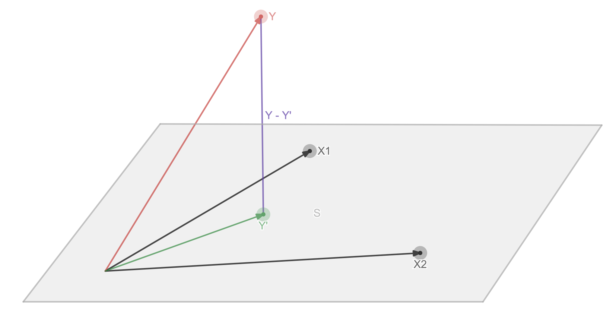
(1) Y -Y 'is vertical with each vector X. The note is M the Mito zero vector

(2) Linear equation that replace Y '

(3) Spread brackets

(4) After moving the item, you can solve W

X T ( y − y ′ ) = 0 ( 1 ) X T ( y − X w ) = 0 ( 2 ) X T y − X T X w = 0 ( 3 ) w = ( X T X ) − 1 X T y ( 4 ) \begin{array}{l} X^{T}\left(y-y^{\prime}\right)=0 & (1) \\ X^{T}(y-X w)=0 & (2)\\ X^{T} y-X^{T} X w=0 & (3) \\ w=\left(X^{T} X\right)^{-1} X^{T} y & (4) \end{array} XT(y−y′)=0XT(y−Xw)=0XTy−XTXw=0w=(XTX)−1XTy​(1)(2)(3)(4)​

You can see that the geometric explanation is consistent with the results of the guidance method

5. Code implementation

Use Python to implement a linear regression algorithm:

def linear(X, y):
    """
    Linear regression
    args:
                 X -Training Data Collection
                 Y -target label value
    return:
                 W -weight coefficient
    """
   # PINV function directly find the pseudo -courses of the matrix
   return np.linalg.pinv(X).dot(y)

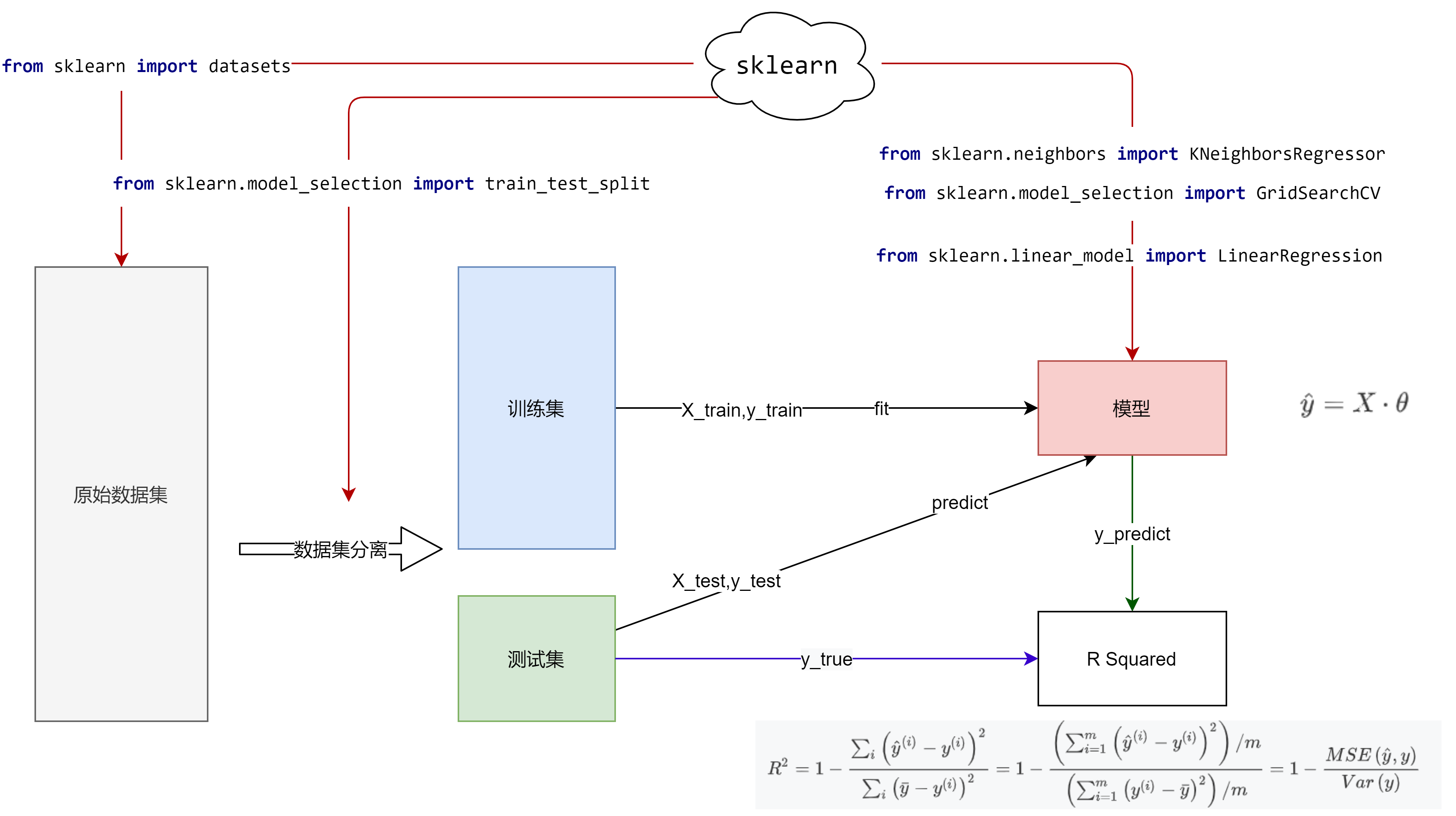
6. Third -party library implementation

scikit-learn⁹ accomplish:

from sklearn.linear_model import LinearRegression

# Initialized linear regression device
lin = LinearRegression(fit_intercept=False)
# Linear model
lin.fit(X, y)
# Weight coefficient
w = lin.coef_

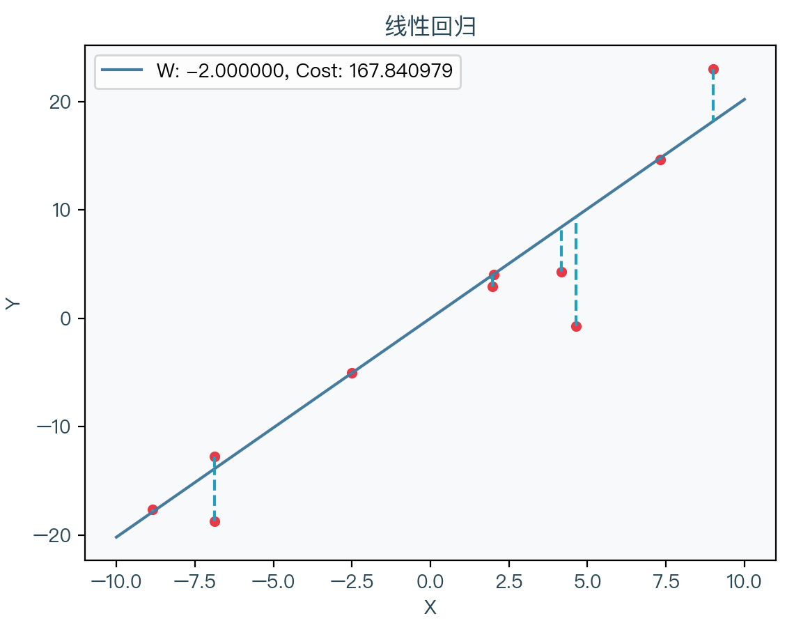
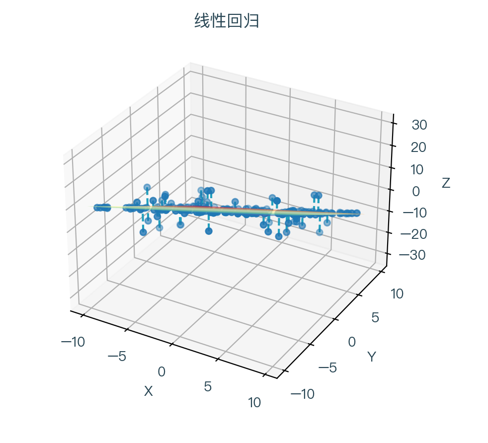
Seven, animation demonstration

When the linear prescription takes different weight coefficients, the corresponding cost function changes can be seen that the cost function is to be reduced to a minimum value and then gradually increased.

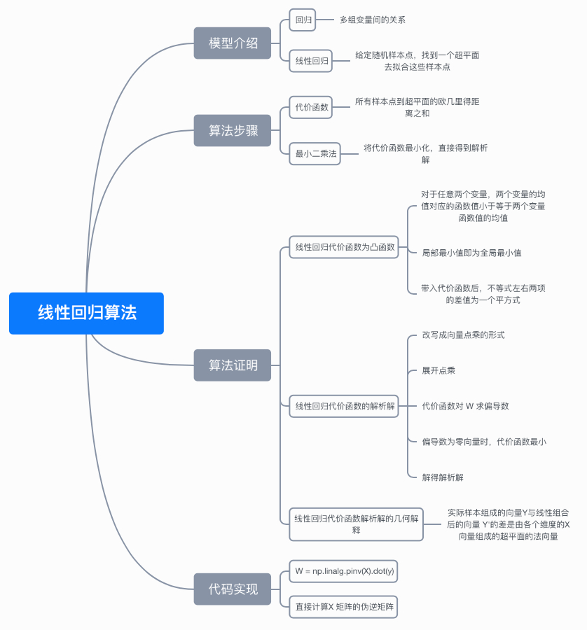
8. Thinking map

9. References

1. https://en.wikipedia.org/wiki/Linear_regression
2. https://en.wikipedia.org/wiki/Euclidean_distance
3. https://en.wikipedia.org/wiki/Arg_max#Arg_min
4. https://en.wikipedia.org/wiki/Convex_function
5. https://en.wikipedia.org/wiki/Transpose
6. https://en.wikipedia.org/wiki/Rank_(linear_algebra)
7. https://en.wikipedia.org/wiki/Multicollinearity
8. https://en.wikipedia.org/wiki/Singular_value_decomposition
9. https://scikit-learn.org/stable/modules/generated/sklearn.linear_model.LinearRegression.html

Please click on a complete demonstrationhere

Note: This article strives to be accurate and easy to understand, but because the author is also a beginner, the level is limited. If there are errors or omissions in the article, readers are requested to criticize and correct them through a message.


This article is first issued in--AI confessionWelcome to follow