Summary of Common Algorithms of "Introduction to Algorithms"
Foreword: Many other blog contents are used in the summary of this article. I originally wanted to attach the original link, but I haven't found it for a long time. The originality here comes from the original author.
Divide and conquer
The idea of divide and conquer strategy:
As the name suggests, divide and conquer is to break down a primitive problem into multiple sub-problems, and the sub-question has the same form as the original question, but the scale is smaller. Through the solution of the sub-question, the original problem will naturally come out. To sum up, it can be roughly divided into three steps:
Decomposition: The original problem is divided into sub-problems of the same form, and the scale can be unequal, divided into half or 2/3 to 1/3.
Solution: For the solution of the sub-problem, it is obvious that the recursive solution is used. If the sub-problem is small enough, the recursion is stopped and solved directly.
Merge: Merges the solution of the subproblem into the solution to the original problem.
Here is a question of how to solve the subproblem, obviously using the recursive call stack. Therefore, the recursive and divide-and-conquer methods are closely linked, and the recursive formula can naturally describe the running time of the divide-and-conquer method. Therefore, if you want to ask me about the relationship between division and recursion, I will answer this: divide and conquer depends on recursion, divide and conquer is an idea, and recursion is a means, recursive can describe the time complexity of divide and conquer algorithm . So introduce the focus of this chapter: How to solve the recursion?
The application of the division and treatment method
The problems that can be solved by the divide and conquer method generally have the following characteristics:
- The scale of the problem is reduced to a certain extent and can be easily solved.
- The problem can be broken down into several smaller, identical problems, ie the problem has the best substructure properties.
- The solution to the subproblem decomposed using this problem can be merged into the solution to the problem;
- The sub-problems decomposed by this problem are independent of each other, that is, sub-problems do not contain public sub-sub-problems.
The first feature is that most problems can be satisfied, because the computational complexity of the problem generally increases as the size of the problem increases;
The second feature is the premise of applying the divide and conquer method. It is also satisfied by most problems. This feature reflects the application of recursive ideas;
The third feature is the key. Whether or not the divide and conquer method can be used depends entirely on whether the problem has the third feature. If it has the first and second features, it does not have the first For three characteristics, you can consider greedy or dynamic programming.
The fourth feature relates to the efficiency of the divide-and-conquer method. If the sub-problems are not independent, the divide-and-conquer method has to do a lot of unnecessary work, and repeatedly solve the public sub-problems. Although the divide and conquer method can be used, it is generally better to use the dynamic programming method.
————————————————————————————————————————————
Maximum heap minimum heap
1, the heap
The heap gives the impression that it is a binary tree, but its essence is an array object, because when the heap is manipulated, the heap is treated as a complete binary tree, and each node of the tree corresponds to the element in the array that holds the value of the node. . So the heap is also called the binary heap. The correspondence between the heap and the complete binary tree is shown in the following figure:

Usually given node i, the node's father node and left and right child nodes can be found according to their position in the array. These three processes are generally implemented by macro or inline functions. When introduced in the book, the subscript of the array starts from 1, and all can be:PARENT(i)=i/2 LEFT(i) = 2i RIGHT(i) = 2i+1
can be divided into the largest heap and the smallest heap based on the conditions that the node values satisfy.
The characteristics of the largest heap are: for each node i except the root node, there is A[PARENT(i)] >= A[i], and the characteristics of the smallest heap are: for each node i except the root node, there is A[ PARENT(i)] >=A[i].
Think of the heap as a tree with the following characteristics:
(1) The height of the heap containing n elements is lgn.
(2) When an array is used to represent a heap storing n elements, the subscripts of the leaf nodes are n/2+1, n/2+2, ..., n.
(3) In the largest heap, the largest element is on the root of the subtree; in the smallest heap, the smallest element is on the root of the subtree.
2, to maintain the nature of the heap
How does a key operation process maintain the unique nature of the heap, given a node i, to ensure that the subtree rooted at i satisfies the heap nature. The book uses the largest heap as an example to illustrate, and gives the recursive form of MAX-HEAPIFY to maintain the maximum stacking operation. Let's look at an example. The operation process is as follows:
It can be seen from the figure that when the node i=2, the maximum heap requirement is not met, and adjustment is needed. The largest one of the left and right children of the node 2 is selected for exchange, and then the checked node i=4 satisfies the maximum heap. The requirements are not satisfied from the diagram, and then adjusted until there is no exchange.
3, build a heap
The process of setting up the largest heap is to call the maximum heap adjuster from bottom to top to turn an array A[1...N] into a maximum heap. Treat the array as a complete binary tree, starting with its last non-leaf node (n/2). The adjustment process is shown below:

4, heap sorting algorithm
The heap sorting algorithm process is: first call the create heap function to make the input array A[1...n] a maximum heap, so that the largest value is stored in the first position of the array A[1], and then the last position of the array is used. A position is swapped and the heap size is reduced by 1, and the maximum heap adjustment function is called to adjust the maximum heap from the first position. The simple process of giving the heap array A={4,1,3,16,9,10,14,8,7} for heap sorting is as follows:
(1) Create the largest heap, the first element of the array is the largest, and the result is as follows:

(2) Loop, from length(a) to 2, and continuously adjust the maximum heap, giving a simple process as follows:

5, the problem
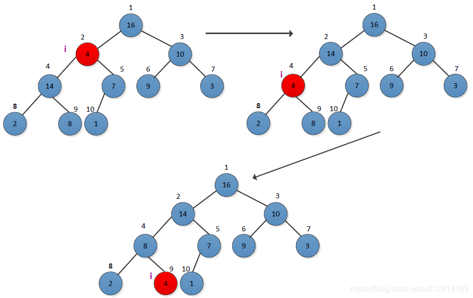
(1) In the process of creating the largest heap, why from the last non-leaf node (n/2) to the end of the first non-leaf, rather than from the first non-leaf node (1) to the last non-leaf node (n/2) End?
My idea is that if you create a heap from the first non-leaf node, it may cause the created heap to not satisfy the nature of the heap, so that the first element is not the largest. This simply makes the node and its left and right child nodes satisfy the heap nature and cannot ensure that the entire tree satisfies the nature of the heap. If the largest node is on a leaf node, it may not appear in the root node. For example, the following example:
As you can see from the figure, the largest heap is created from the first non-leaf node, and the final result is not the largest heap. When the heap is created from the last non-leaf node, it can be guaranteed that the subtree of the node satisfies the nature of the heap, so that the heap is adjusted from the bottom up, and finally the maximum heap property is satisfied.
6. Summary:
1. Adjust the maximum heap time complexity: O (lgn)
2. build heap, because the height of each comparison is actually not large, so for an unordered array n, the time complexity of constructing it into the largest heap is O(n), which is a linear time complexity.
3. Use the largest heap method to sort an unordered data, the time complexity is O(n+n*lgn)=O(nlgn)
4. For the maximum heap build, the main thing to do is to start the build from the last non-leaf node up (array forward) to build the heap, the purpose of this is to allow the maximum data of the leaf node to pass. Adjust to the root node.
If the heap is started from the first root node, then if the largest node is at the leaf node, this adjustment will not result in the maximum data being adjusted to the root node, because only the current node can be guaranteed. And the size of the leaf node is adjusted, the node of the root node is adjusted, and then there is no adjustment.
————————————————————————————————————————————
Priority queue
A queue is a data structure that satisfies a first-in, first-out (FIFO) data. Data is taken from the head of the queue. New data is inserted from the end of the queue. The data is equal and there is no priority. This is similar to ordinary people going to the train station to queue up to buy tickets. The first to buy tickets first, each person is equal, there is no priority right, the whole process is fixed. Priority queues can be understood as assigning a weight to each data on a queue basis, representing the priority of the data. Similar to the queue, the priority queue also extracts data from the header and inserts data from the tail. However, this process varies according to the priority of the data. It always comes first with high priority, so it is not necessarily FIFO. This is similar to when a train ticket is bought by a soldier. The military is better than the average person. Although the military comes late, the priority of the soldier is higher than that of the average person. It is always possible to buy the ticket first. Usually the priority queue is used for multi-task scheduling in the operating system. The higher the priority of the task, the priority of the task (similar to the out-of-queue), and the later tasks need to adjust the task to the appropriate position if the priority is higher than the previous one. In order to prioritize execution, the entire process always makes the first task of the task in the queue have the highest priority.
There are two types of priority queues: the maximum priority queue and the minimum priority queue, which can be implemented with the largest heap and the smallest heap, respectively. The book describes the maximum priority queue based on the maximum heap implementation. The operations supported by a maximum priority queue are as follows:
INSERT(S,x): insert the element x into the set S
MAXIMUM(S): Returns the element with the largest keyword in S
EXTRACT_MAX(S): Remove and return the element with the largest keyword in S
INCREASE_KEY(S, x, k): Increases the value of the key of element x to k, where the value of k cannot be less than the value of the original key of x.
problem
How to use a priority queue to implement a first in first out queue and a advanced outbound stack?
My idea is that the elements in the queue are first in, first out (FIFO), so the queue can be implemented with the smallest priority queue. The specific idea is to assign a weight to each element in the queue, and the weight is incremented from the first element to the last one (if the array is implemented, the subscript in which the element is located can be used as the priority, and the priority is small. First out queue), the element dequeue operation takes the first element of the priority queue each time. After the completion, the heap minimum priority queue needs to be adjusted to make the first element have the lowest priority. The elements in the stack are just the opposite of the queue. The element is advanced out (FILO), so it can be implemented with the highest priority queue. Similar to the idea of implementing queues with the smallest priority queue, the priority of the marked elements is in the order in which they appear. The more the data is, the higher the priority.
An example of implementing a FIFO queue with a minimum priority queue, now has a set of numbers A={24,15,27,5,43,87,34} for a total of six numbers, assuming The array subscript starts at 1, and the priority queue is created with the subscript in the array of the element as the priority. The minimum priority queue is adjusted when the elements in the queue go in and out. The operation process is as shown in the following figure:

"Introduction to Algorithms After Class Exercises"
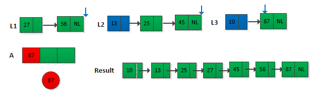
The topic is as follows: Please give an algorithm for time O(nlgk), which is used to combine k sorted linked lists into one sorted linked list. Here n is the total number of elements in all input linked lists. (Hint: use a minimum heap to do k-way merge).
The first thing I see when I see the problem is the sub-process of the merge operation in the merge sorting process. I start from the beginning to compare the two, find the smallest one, and then compare it later. The common one is the 2-way merge. The title is given to k ordered lists (k>=2). If there is no prompt, I don't know how to implement it for a long time. Fortunately, I am prompted to use the smallest heap to do k-way merge, so I thought I could do this:Create an array of size k, store the first element in the k linked list into the array, and then adjust the array to the smallest heap, so that the first element of the array is the smallest, assuming min, will min Take the smallest heap and store it in the linked list of the final result. At this point, put the next element of the linked list in min into the smallest heap inserted, and continue the above operation until there are no elements in the heap.. An example is shown below (only some operations are given):

The final result is shown below:
to sum up:
For a prioritized unordered event, the queue is entered and exited in order of priority, and the time complexity of implementation is O(lgn)
————————————————————————————————————————————
Linear time ordering
There are three main sorting algorithms for algorithm linear time, counting sorting, cardinal sorting, and bucket sorting. They do not need to compare operations, they are sorted by the position of the elements themselves, and thus require additional storage idle, but can have linear time complexity O(n). At the same time, all three sorting algorithms are stable.
Count sort
Just use an extra array to record the number of occurrences of each element, and use the Fibonacci idea to add the sequential time, then you can find out how many elements are in front of each element, and finally follow this Additional arrays can be placed directly in the corresponding location.
Count sorting assumes that each of the n input elements is an integer between 0 and k, and k is the largest of the n numbers. When k=O(n), the running time of the counting order is θ(n). The basic idea of counting sorting is: for each element x of n input elements, the number of elements less than or equal to x is counted, and the final position of x in the output array can be determined according to the number of x. This process needs to introduce two auxiliary storage spaces, storing the result B[1...n], and an array C[0...k] for determining the number of each element.
The specific steps of the algorithm are as follows:
(1) Determine the value of k according to the value of the element in the input array A, and initialize C[1...k]= 0;
(2) Traverse the elements in the input array A, determine the number of occurrences of each element, and store the number of occurrences of the ith element in A in C[A[i]] Medium, then C[i]=C[i]+C[i-1], and it is determined in C that there are multiple elements in front of each element in A;
(3) Reverse the elements in array A in reverse order, find the number of occurrences in A in C, and determine the position in array B, and then reduce the number of times in C. 1.
An example is given to illustrate the process. Assume that the input array A=<2,5,3,0,2,3,0,3>, the sorting process is as follows:

Cardinality sort
According to the size of the base, sorting from low to high is first sorted according to the lower order of the element. On the sorted sequence, the order is sorted according to the high order of the elements, and the order is sorted from low to high once, and the final sort is completed. The low order is performed in sort order.
The cardinal sorting process does not need to compare keywords, but through the "allocation" and "collection" processes to achieve sorting, its time complexity can reach linear order: O (n). For decimal numbers, each bit in [0,9], the number of d bits, has a d column. The cardinality sorting is first sorted by the lower significant digits, and then the next digit is sorted one by one until the highest rank order ends.
An example of the cardinality sorting process is shown in the following figure:

The cardinality sorting algorithm is very straightforward. Assume that in array A of length n, each element has a d-bit number, where the first bit is the lowest bit and the d-th bit is the highest bit.
Bucket sort
It is relatively simple, that is, the sequence to be divided into different sections, each section is treated as a bucket, which is sorted first in its own bucket, and then the data of each bucket is connected together. But this requires extra overhead.
Count sorting assumes that the input is composed of a small integer, while bucket sorting assumes that the input is generated by a random process that distributes the elements evenly and independently over the interval [0] , 1) on. When the bucket sorted input conforms to a uniform distribution, it can run at a linear desired time. The idea of bucket sorting is to divide the interval [0, 1) into n sub-intervals of the same size, into a bucket, and then distribute the n input numbers to each bucket to sort the numbers in each bucket. And then list the elements in each bucket in order.
to sum up
The linear time sorting method has an increase in time complexity relative to the comparison sorting, but at the same time it is necessary to sacrifice additional space overhead, which is also normal.
————————————————————————————————————————————
Median and sequential statistics
The problem discussed in this chapter is to select the ith order statistic problem in a set of n different values. The main content is how to select the i-th small element in the set S in the O(n) time in the linear time. The most basic is to select the maximum and minimum values of the set. In general, the selected elements are random, and the maximum and minimum values are special cases. The book focuses on how to use the divide-and-conquer algorithm to select the i-th small element and optimize it with the median to ensure the worst. Ensure that the runtime is linear O(n).
1, the basic concept
Order statistic: In a set of n elements, the ith order statistic is the ith smallest element in the set. For example, the minimum value is the first sequential statistic, and the maximum value is the nth sequential statistic.
Median: In general, the median refers to the "intermediate element" of the set it is in. When n is odd, the median is unique and the occurrence position is n/ 2; When n is even, there are two medians, the positions are n/2 (upper median) and n/2+1 (lower median).
2, select the problem description
Input: A set A containing n (different) numbers and a number i, 1 ≤ i ≤ n.
Output: Element x∈A, which is just larger than the other i-1 elements in A.
The most straightforward way is to use a sorting algorithm to sort the set A first, and then output the i-th element. You can use the merge sort, heap sort, and quick sort as mentioned above, and the running time is O(nlgn). In the following book, I will explain how to solve this problem in linear time from shallow to deep.
The general choice problem seems to be more difficult than choosing the maximum and minimum values, but the running time of the two problems is the same, both θ(n). Introduced in the bookThe divide-and-conquer algorithm is used to solve the general selection problem, and the process is similar to the division in the fast sorting process.. Each time the set is divided, the final position of an element can be determined. According to this position, it can be judged whether it is the i-th small element we require. If not, then we only care about dividing one of the two sub-parts of the output, judging whether it is the previous or the latter according to the value of i, and then dividing the sub-array, repeating the process until the i-th small is found. element. The partitioning can be done randomly, which ensures that the expected time is θ(n) (assuming all elements are different).
Give an example to illustrate this process, assuming that the existing set A = {32, 23, 12, 67, 45, 78, 10, 39, 9, 58}, requires its fifth small element, assuming total in the division process The last element is divided into main elements. The execution process is as follows:
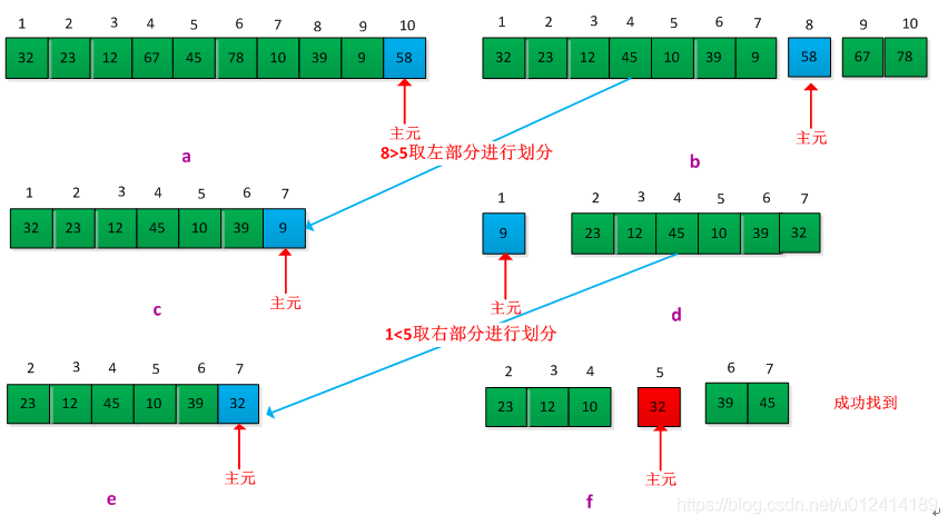
The selection algorithm in this chapter has linear run time because these algorithms are not sorted, and the linear time behavior is not the result of making assumptions about the input.
————————————————————————————————————————————
Hash list
This chapter introduces the concept of hash tables, the design of hash functions, and the handling of hash collisions. The hash table is similar to the dictionary directory. The searched elements all have a key corresponding to it. In practice, the efficiency of the hashing technique is very high. A reasonable design of the scatter function and the conflict handling method can make the lookup in the hash table. The expected time of an element is O(1). The hash table is a generalization of the concept of ordinary arrays. In the hash table, instead of directly using the keyword as an array subscript, it is calculated based on the keyword through a hash function. The function of the map container in STL is the function of the hash table, but the map is implemented by the red-black tree, followed by learning.
1, direct addressing table
When the global (range) U of the keyword is relatively small, direct addressing is a simple and effective technique. Generally, an array can be used to implement a direct addressing table. The array subscript corresponds to the value of the keyword, that is, has the keyword k. The elements are placed in slot k of the direct addressing table. The dictionary operation of the direct addressing table is relatively simple to implement, and the array can be directly manipulated, and only O(1) time is required.
2, hash table
The disadvantage of the direct addressing table is that when the range U of the keyword is large, it is not practical to construct a table storing the size of |U| under the limitation of the memory capacity of the computer. When the set of keywords K stored in the dictionary is much smaller than all possible key fields U, the hash table requires much less storage space than the direct addressing table. The hash table calculates the position of the key k in the slot by the hash function h. The hash function h maps the key field U to the slot of the hash table T[0...m-1]. That is, h:U->{0,1...,m-1}. The purpose of using a hash function is to reduce the size of the small size that needs to be processed, thereby reducing the overhead of the space.
There is a problem with the hash table: the two keywords may be mapped to the same slot, ie collision. Need to find an effective way to resolve the collision.
3, the hash function
A good hash function is characterized by the fact that each keyword is hashed to any of the m slots and is independent of which slot the other keywords have been hashed into. Most hash functions assume that the key fields are natural numbers N={0,1,2,...}. If the given keywords are not natural numbers, there must be a way to interpret them as natural numbers. For example, when the keyword is a string, it can be converted to a natural number by adding the ASCII code of each character in the string.
The book introduces three design schemes: the division hash method, the multiplication method, and the global hash method.
(1) Divisional hashing
The key k is mapped to one of the m slots by taking the remainder of k divided by m. The hash function is: h(k) = k mod m . m should not be a power of 2, usually the value of m is a prime number that is not too close to the integer power of 2.
(2) Multiplication hashing
This method is not very clear when you look at it. If you don't figure out what it means, first record the basic thoughts and digest it in the future. Constructing a hash function by multiplication hashing requires two steps. In the first step, the constant k is multiplied by the keyword k (0 < A < 1), and the fractional part of kA is extracted. Then, multiply this value by m and take the bottom of the result. The hash function is as follows: h(k) = m(kA mod 1).
(3) Global hash
Given a set of hash functions H, a hash function h is randomly selected from H each time a hash is made, such that h is independent of the key to be stored. The average performance of the global hash function class is better.
4, collision processing
There are usually two ways to handle collisions:Open Addressing and Chaining. The former is to store all nodes in the hash table T[0...m-1]; the latter usually puts all the elements hashed into the same slot in a linked list, and puts the head pointer of this linked list In the hash table T[0...m-1].
(1) Open addressing method
All elements are in the hash table, each table item or an element containing a dynamic collection, or contains NIL. In this method the hash table may be filled so that no new elements can be inserted. In the open addressing method, when an element is to be inserted, the items of the hash table can be continuously checked or detected until there is an empty slot to place the keyword to be inserted. There are three techniques for open addressing: linear detection, secondary detection, and dual detection.
<1>Linear detection
Given a normal hash function h':U ->{0,1,...,m-1}, the hash function used by the linear detection method is:h(k,i) = (h’(k)+i)mod m,i=0,1,…,m-1
When detecting from i=0, first probe T[h'(k)], then detect T[h'(k)+1],... in turn, until T[h' (k) + m-1], and then loop to T[0], T[1], ... until T[h'(k)-1] is detected. The detection process ends in three cases:
(1) If the currently detected unit is empty, it means that the search failed (if it is inserted, the key is written into it);
(2) If the currently detected unit contains a key, the search is successful, but it means failure for insertion;
(3) If no empty cell is found and no key is found when T[h'(k)-1] is detected, neither search nor insert means failure (at this time) Table full).
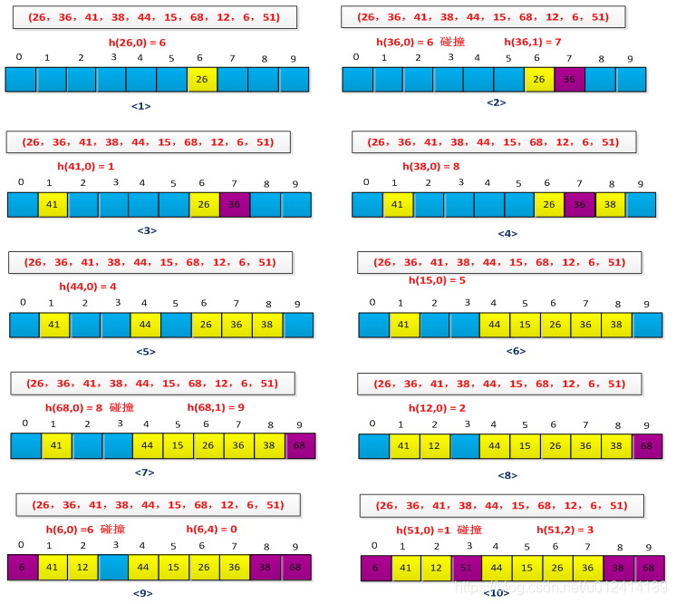
The linear detection method is easier to implement, but there is a clustering problem where the sequence of consecutively occupied slots becomes longer and longer. An example is used to illustrate the linear detection process. A set of keywords is known as (26, 36, 41, 38, 44, 15, 68, 12, 6, 51). The hash function is constructed by the remainder method. The initial situation is as follows. Shown as follows:
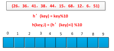
The hashing process is shown below:
<2>Secondary detection
The probe sequence of the second detection method is: h(k, i) = (h'(k) + i*i)%m, 0 ≤ i ≤ m-1. The initial detection position is T[h'(k)], and the subsequent detection position is added with an offset on the basis of the second, and the offset depends on i in a quadratic manner. The drawback of this method is that it is not easy to detect the entire hash space.
<3>Double hash
This method is one of the best methods of open addressing because it produces an array with many features of a randomly chosen arrangement. The hash function used is: h(k,i)=(h1(k)+ih2(k)) mod m. Where h1 and h2 are auxiliary hash functions. The initial detection position is T[h1(k)], and the subsequent detection position is added to the offset h2(k) modulo m.
(2) Link method
Link all nodes whose synonyms are synonymous in the same linked list. If the selected hash table length is m, the hash table can be defined as an array of pointers T[0...m-1] consisting of m header pointers. Any node whose hash address is i is inserted into a singly linked list with T[i] as the head pointer. The initial value of each component in T should be a null pointer. In the zipper method, the filling factor α can be greater than 1, but generally takes α ≤ 1.
For example, the execution process of the link method is set up with a set of keywords (26, 36, 41, 38, 44, 15, 68, 12, 6, 51). The hash function is constructed by the remainder method. The initial situation is as shown in the figure below. Show:
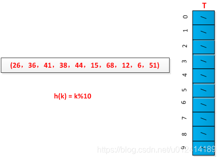
The final result is shown below:

5, string hash
Usually the key of the element is converted to a number for hashing. If the key itself is an integer, then the hash function can use keymod tablesize (to ensure that tablesize is a prime number). In actual work, strings are often used as keywords, such as body names, positions, and so on. At this time, you need to design a good hash function process to process the element whose keyword is a string.
There are several ways to deal with it:
method 1: Adds the ASCII code values of all the characters of the string, and takes the resulting sum as the key of the element. The hash function of the design is as follows:
1 int hash(const string& key,int tablesize)
2 {
3     int hashVal = 0;
4     for(int i=0;i<key.length();i++)
5            hashVal += key[i];
6     return hashVal % tableSize;
7 }
The disadvantage of this method is that the elements cannot be effectively distributed. For example, if the keyword is a string of 8 letters, the length of the hash table is 10007. The maximum ASCII code of the letter is 127. According to the method 1, the maximum value corresponding to the keyword is 127×8=1016, which means that only the slot 0-016 of the hash table can be mapped through the hash function mapping. As a result, most of the grooves are not used, the distribution is uneven, and the efficiency is low.
Method 2: Suppose the keyword consists of at least three letters, and the hash function simply hashes the first three letters. The hash function of the design is as follows:
1 int hash(const string& key,int tablesize)
2 {
3         //27 represents the number of letters plus the blank
4         return (key[0]+27*key[1]+729*key[2])%tablesize;
5 }
This method simply hashes the ASCII code of the first three characters of the string. The maximum value obtained is 2851. If the length of the hash is 10007, only 28% of the space is used. Most of the space is not used. . So if the hash table is too large, it doesn't work.
Method 3: Construct a prime (usually 37) polynomial with the help of Horner's rules (very clever, don't know why it is 37). The calculation formula is: key[keysize-i-1]37^i, 0<=i<keysizesum. The hash function of the design is as follows:
 1 int hash(const string & key,int tablesize)
 2 {
 3         int hashVal = 0;
 4         for(int i =0;i<key.length();i++)
 5             hashVal = 37*hashVal + key[i];
 6         hashVal %= tableSize;
   7 if(hashVal<0) //calculated hashVal overflow
 8            hashVal += tableSize;
 9        return hashVal;
10 }
The problem with this method is that if the string keyword is long, the calculation process of the hash function becomes longer, which may cause the calculated hashVal to overflow. For this case, some characters of the string can be calculated, for example, characters of even or odd bits are calculated.
6, rehashing - re-hashing can ensure that the average search complexity does not become
If the hash table is full, it will fail when you insert a new element into the hash table. At this time, another hash table can be created, so that the length of the new hash table is more than twice that of the current hash table, and the hash value of each element is recalculated and inserted into the new hash table. The question of re-hashing is when is the best, there are three cases to determine whether to re-hash:
(1) When the hash table is about to be full, given a range, for example, the hash has been used up to 80%, this time to re-hash.
(2) When a new element fails to be inserted, it is hashed again.
(3) According to the loading factor (the hash table T with n slots for n elements, the loading factor α=n/m, ie the average storage in each chain) The number of elements is judged, and when the load factor reaches a certain threshold, it is performed in the hash.
When using the link method to deal with collision problems, the third method is the best in hashing efficiency.
————————————————————————————————————————————
Red black tree
The red-black tree is a binary search tree, but a storage bit is added to each node to indicate the color of the node, which can be RED or BLACK. By limiting the coloration of any path from root to leaf, the red-black tree ensures that no path is twice as long as other paths and is therefore nearly balanced. This chapter mainly introduces the nature of red and black trees, left and right rotation, insertion and deletion. The process of inserting and deleting elements in the red-black tree is analyzed in detail, and the situation is discussed in detail. A binary search tree of height h can implement any basic dynamic set operation, such as SEARCH, PREDECESSOR, SUCCESSOR, MIMMUM, MAXMUM, INSERT, DELETE, and so on. These operations perform faster when the height of the binary search tree is lower, but when the height of the tree is higher, the performance of these operations may be no better than using a linked list. The red-black tree is a balanced binary search tree that guarantees that the basic dynamic operation set runtime is O(lgn) in the worst case. The content of this chapter is somewhat complicated. After two days of reading, I will probably understand the process of inserting and deleting. I need to review it frequently in the future and try to completely digest it. Red-black trees are very versatile. For example, the map in STL is implemented in red-black trees. It is very efficient and has the opportunity to study the source code of STL.
1. The nature of red and black trees
Each node in the red-black tree contains five fields: color, key, left, right, and parent. If a node does not have a child node or a parent node, the corresponding pointer parent field of the node contains a value of NIL (NIL is a null pointer, which is somewhat confusing, explained later). Think of NIL as a pointer to the outer node (leaf) of the red-black tree, and the node with the keyword as the inner node of the red-black tree. The red-black tree node structure is as follows:
 1 #define RED  0
 2 #define BLACK 1
 3 struct RedBlackTreeNode
 4 {
 5     T key;
 6     struct RedBlackTreeNode * parent;
 7     struct RedBlackTreeNode * left;
 8     struct RedBlackTreeNode * right;
 9     int color;
10 };
The nature of the red-black tree is as follows:
(1) Each node is either red or black.
(2) The root node is black.
(3) Each leaf node (NIL) is black.
(4) If a node is red, its two sons are black.
(5) For each node, all paths from the node to its grandchild node contain the same number of black nodes.
The picture below is a red-black tree:
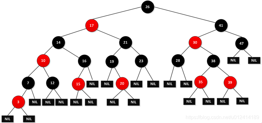
It can be seen from the figure that NIL is not a null pointer, but a leaf node. In actual operation, the NIL can be regarded as a sentinel, which is convenient for operating in black and red. The operation of the red-black tree is mainly for the internal node operation, because the internal node stores the value of the keyword. In the book, for the sake of discussion, the leaf nodes are ignored. If the red and black trees in the above picture become as shown below:

The book gives the concept of black height:Starting from a node x (excluding the node) to any path of a leaf node, the number of black nodes is called the black height of the node.. It can be seen from the nature of the red-black tree (5) that all descending paths from the node have the same number of black nodes. The black height of a red-black tree is defined as the black height of its root node.
A lemma is given in the book to explain why red-black trees are a good search tree and prove the lemma (proven by inductive method, it needs to be strong The knowledge of inductive reasoning is my shortcoming, and the pain of reading is here.)
Lemma: The height of a red-black tree with n inner nodes is 2lg(n+1).
Comparison and doubt:
1. The difference and connection between red black tree and balanced binary tree (AVL tree)
2. The red-black tree adds the inserted node to the red node.
3. Where is the red-black tree used? How does it compare to other balanced search trees?
answer:
1, red-black trees do not pursue "complete balance" - it only requires partial balance requirements, reducing the need for rotation, thereby improving performance.
Red-black trees can search, insert, and delete operations with O(log2 n) time complexity. In addition, due to its design, any imbalance will be resolved within three rotations. Of course, there are some better, but more complex data structures that can be balanced within a single rotation, but red-black trees can give us a "cheap" solution. The algorithm time complexity of the red-black tree is the same as AVL, but the statistical performance is higher than the AVL tree.
Balance the strict height control of the binary tree. The height difference between the left and right subtrees cannot be greater than 1. This causes the insertion and deletion to have more rotation adjustment steps, and the height of the tree must be lgn, which means that the average time of the tree is complicated. Degree is O(lgn)
But the red-black tree only guarantees that any node to leaf node contains the same number of black nodes, and the shape of the tree is constrained by color. The main features are as follows:
1. The height of the red-black tree is always lower than 2lg(n+1), and n is the number of nodes.
2. The time complexity of the red-black tree is O(h(x))= O(2lg(n+1))=O(lgn)
3. Any imbalance caused by insert deletion can be balanced within three rotations, reducing the complexity of the implementation.
If you find more, you can choose to use avltree, insert more deletes, you can use rbtree.
1, black, if it is black, then no matter what the original red and black tree is, it will definitely break the balance.Because the original tree is balanced, now there is a black on this path, which inevitably violates the nature of 5 (when you don't remember, look at it several times and understand it is the best).
2, red,If the newly inserted point is red, it may also break the balance, mainly because it violates the property 4. For example, in the above figure, the parent node 22 of the newly inserted point 21 is red. But there is a special case, such as the above picture, if I insert a node with key=0. Setting the 0 node to red does not affect the balance of the original tree, because the parent node of 0 is black.
as shown below:

Well, there is no need to adjust, so you still choose to set the newly inserted node color to red.
AVL tree
Balanced binary tree is generally determined by the difference of the balance factor and is realized by rotation. The height difference between the left and right subtrees is not more than 1, so it is a strict balanced binary tree compared with the red black tree, and the equilibrium condition is very strict (the height difference is only 1). ), as long as the insertion or deletion does not satisfy the above conditions, it is necessary to maintain balance by rotating. Because the rotation is very time consuming. We can launch AVL treeIt is suitable for the case where the number of insertions and deletions is relatively small, but there are many searches.
The application is relatively small compared to other data structures. Windows manages the process address space using the AVL tree.
Red-black tree: Balancing a binary tree, by constraining the color of each node on any simple path from root to leaf, ensuring that no path is twice as long as other paths and is therefore approximately balanced. Therefore, it is less balanced in rotation than the AVL tree, which is strictly required to be balanced. When used for searching, we use a red-black tree instead of AVL when there are many insertions and deletions.
Red black trees are widely used:
· Widely used in C++'s STL. Both map and set are implemented in red and black trees.
· The well-known Linux process schedules the Completely Fair Scheduler, which manages the process control block with a red-black tree.
· Implementation of epoll in the kernel, managing event blocks with red and black trees
· nginx, use red and black trees to manage timers, etc.
· Java TreeMap implementation
B-tree, B+ tree: They have the same characteristics. They are multi-way search trees. They are generally used for indexing in databases because they have fewer branches, because disk IO is very time consuming, and like large amounts of data are stored on disk. So we have to effectively reduce the number of disk IOs to avoid frequent disk lookups.
The B+ tree is a variant tree of the B-tree. The nodes with n subtrees contain n keywords. Each keyword does not store data, but is used only for indexing, and the data is stored in the leaf node. It was born for the file system.
The B+ tree is less expensive to read and write than the B-tree disk: because the B+ tree non-leaf nodes only store key values, the single node occupies less space, the index block can store more nodes, and the index blocks needed to read the index from disk are more Less, so the number of I/Os in the index lookup is less than that of the B-Tree index, and the efficiency is higher. And the records that B+Tree stores in the leaf nodes are linked in the form of a linked list.Range lookup or traversal is more efficient. Mysql InnoDB uses the B+Tree index.
Trie Tree:
Also known as word search tree, a tree structure, commonly used to manipulate strings. It is only one copy of the same prefix for different strings.
Relatively saving a string is definitely space-saving, but it saves memory (is memory) when it saves a large number of strings.
Similar to: prefix tree, suffix tree, radix tree (flatcia tree, compactprefix tree), crit-bit tree (solving memory problems), and The double array trie mentioned earlier.
Prefix tree: fast string retrieval, string sorting, longest common prefix, automatic matching prefix display suffix.
Suffix tree: Find the number of times string s1 is in s2, the number of occurrences of string s1 in s2, the longest common part of string s1, s2, and the longest palindrome.
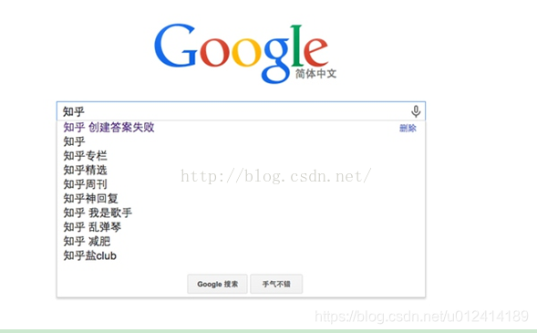
A typical application for the trie tree is prefix matching, such as the very common scenario below, where the search engine gives hints as we type. Also, for example, IP routing, but also prefix matching, will use trie to some extent.
Red and black trees often ask questions during the interview
1. What data structure is used in the set of the set in stl?
2. How is the data structure of the red-black tree defined?
3. What are the properties of red and black trees?
4. What is the time complexity of the various operations of the red-black tree?
5. What are the advantages of red-black trees compared to BST and AVL trees?
6. What is the basis for the red-black tree relative to the hash table when it is selected for use?
7. How do you extend the red-black tree to get more elements than a node?
8. What are the steps to extend the data structure?
9 Why is the number of buckets in a typical hashtable taking a prime number?
Detailed answer
1. What data structure is used in the set of the set in stl?
Red black tree
2. How is the data structure of the red-black tree defined?
 1. enum Color
 2. {
 3.           RED = 0,
 4.           BLACK = 1
 5. };
 6.
 7. struct RBTreeNode
 8. {
 9.            struct RBTreeNode*left, *right, *parent;
 10.            int   key;
 11.            int data;
 12.            Color color;
 13. };
3. What are the properties of red and black trees?
In general, red-black trees satisfy the following characteristics, that is, only trees that satisfy all of the following properties are called red-black trees:
1) Each node is either red or black.
2) The root node is black.
3) Each leaf node (the leaf node refers to the NIL pointer or NULL node at the end of the tree) is black.
4) If a node is red, then its two sons are black.
5) For any node, each path to the NIL pointer at the end of the leaf node tree contains the same number of black nodes.
4. What is the time complexity of the various operations of the red-black tree?
It can guarantee that in the worst case, the basic dynamic geometry operation time is O(lgn)
5. What are the advantages of red-black trees compared to BST and AVL trees?
Red black tree isAt the expense of the rigorously high balance of superior conditions, it only requires partial balancing requirements, reducing the need for rotation and thus improving performance. Red-black trees can search, insert, and delete operations with O(log2 n) time complexity. In addition, due to its design, any imbalance will be solved within three rotations.. Of course, there are some better, but more complex data structures that can be balanced within a single rotation, but red-black trees can give us a "cheap" solution.
Compared to BST, because the red-black tree can ensure that the longest path of the tree is no more than twice the length of the shortest path, it can be seen that its search effect is guaranteed to be minimal. In the worst case, O(logN) can also be guaranteed, which is better than the binary search tree. Because the worst case of the binary search tree allows the lookup to reach O(N).
The algorithm time complexity of the red-black tree is the same as that of the AVL, but the statistical performance is higher than the AVL tree, so the post-maintenance operations in the insert and delete will definitely take much longer than the red-black tree, but their search efficiency is It is O(logN), so the red-black tree application is still higher than the AVL tree. The speed of inserting the AVL tree and the red-black tree depends on the data you insert. If your data is well distributed, it is better to adopt. AVL tree (for example, randomly generating series numbers), but if you want to deal with the messy situation, the red black tree is faster.
6. What is the basis for the choice of red and black trees relative to the hash table when using it?
Weigh three factors: == speed of discovery, amount of data, memory usage, scalability. ==
In general, the hash lookup speed is faster than the map, and the search speed is basically independent of the data size, which is a constant level; and the map search speed is log(n) level. It doesn't necessarily mean that the constant is smaller than log(n). The hash and the hash function take time. Understand it. If you consider efficiency, especially when the element reaches a certain order of magnitude, consider considering the hash.But if you are particularly strict with memory usage and want the program to consume as little memory as possible, then be careful, hashes can make you jealous, especially when your hash object is particularly large, you are even more uncontrollable, and the hash The construction speed is slower.
Red-black trees do not fit into the realm of all application trees. If the data is basically static, let them stay in place where they can insert and do not affect the balance. If the data is completely static, for example, to make a hash table, performance may be better.
In an actual system, for example,Firewall systems that require dynamic rules, using red-black trees instead of hash tables have proven to be more scalable. The Linux kernel uses a red-black tree to maintain memory blocks when managing vm_area_struct.
The red-black tree can be used to extend the node domain to get the rank of the node without changing the time complexity.
7. How to expand the red-black tree to get more elements than a node?
This is actually the order statistic of the node elements. Of course, any order statistic can be determined within O(lgn) time.
Add a size field to each node to represent the size of the node tree of the subtree rooted at node x
is theresize[x] = size[[left[x]] + size [right[x]] + 1;At this time, the red-black tree becomes a sequential statistical tree.
There are two things you can do with the size field:
1). Find the i-th small node in the tree;
 1. OS-SELECT(x;,i)
 2. r = size[left[x]] + 1;
 3. if i == r
 4.      return x
 5. elseif i < r
 6.      return OS-SELECT(left[x], i)
 7. else return OS-SELECT(right[x],  i)
Idea: size[left[x]] indicates the number of pre-x traversal in the sub-tree traversing x, and the depth of recursive calls will not exceed O(lgn);
2). Determine how many nodes before a node, that is, the problem we want to solve;
 1. OS-RANK(T,x)
 2. r = x.left.size + 1;
 3. y = x;
 4. while y != T.root
 5.          if y == y.p.right
 6.                  r = r + y.p.left.size +1
 7.          y = y.p
 8. return r
Idea: The rank of x can be regarded as the traversal of the order in the tree, and the number of nodes before x is added to one. In the worst case, the OS-RANK runtime is proportional to the tree height, so it is O (lgn).
8. What are the steps to extend the data structure?
1). Select the basic data structure;
2). Determine what information to add in the underlying data structure;
3). Verify the basic modification operations available on the underlying data structure to maintain these newly added information;
4). Design new operations.
9 Why is the number of buckets in a general hashtable taking a prime number?
Has a hash function
H( c ) = c % N;
When N takes a composite number, the simplest example is to take 2n, say 23=8, this time
H( 11100(binary) ) = H( 28 ) = 4
H( 10100(binary) ) = H( 20 )= 4
At this time, the 4th digit of c (from right to left) is "failed", that is, regardless of the value of the 4th bit of c, the value of H(c) is the same. At this time, the fourth position of c does not participate in the operation of H(c) at all, so that H(c) cannot completely reflect the characteristics of c, increasing the probability of causing conflicts.
When taking other combinations, it will cause some bits of c to "fail" to varying degrees, causing conflicts in some common applications.
But taking primes basically ensures that every bit of c participates in H(c) operations, reducing the chance of collisions in common applications.
———————————————————————————————————————————
Dynamic programming
Solve the whole problem by combining the solutions of the sub-problems. The divide-and-conquer algorithm refers to dividing the problem into independent sub-problems, recursively solving each problem, and then merging the solutions of the sub-problems to obtain the solution of the original problem. For example, merge sorting, fast sorting is based on the idea of divide and conquer algorithm.
Dynamic programming differs from this in that sub-problems are not independent, meaning that sub-problems contain common sub-problems. In this case, the divide-and-conquer algorithm will repeat unnecessary work.Use the dynamic programming algorithm to solve each sub-question only once, and store the results in a table.For later sub-questions, to avoid recalculating the answer each time you encounter each sub-question.
The difference between dynamic planning and divide and conquer:
(1) Divide and conquer method refers to dividing the problem into independent sub-problems and recursively solving sub-problems
(2) Dynamic programming applies to situations where these subproblems are not independent, ie subproblems contain common subproblems
Dynamic programming is often used to optimize problems (such problems generally have many feasible solutions, and we hope to find a solution with the best (maximum or minimum) value from these solutions). The design of the dynamic programming algorithm is divided into the following four steps:
(1) Structure describing the optimal solution
(2) Recursively define the value of the optimal solution
(3) Calculate the value of the optimal solution in a low-upward manner
(4) Construct an optimal solution from the calculated result
1, the basic concept
Dynamic programming solves the whole problem by combining the solutions of sub-problems. By decomposing the problems into sub-problems that are not independent of each other (each sub-question contains a common sub-problem, also called an overlapping sub-problem), each sub-question is solved once. Save the results to a secondary table to avoid recalculation each time you encounter a sub-question. Dynamic planning is often used to solve optimization problems.
The design steps are as follows:
(1) Describe the structure of the optimal solution.
(2) Recursively define the value of the optimal solution.
(3) Calculate the value of the optimal solution in a bottom-up manner.
(4) Construct an optimal solution from the calculated result.
The first step is to choose the optimal solution when the problem occurs. By analyzing the optimal solution of the sub-problem, the optimal solution to the whole problem is achieved. In the second step, according to the optimal solution description obtained in the first step, the whole problem is divided into small problems until the problem can no longer be divided, the layer selection is optimal, and the optimal solution of the whole problem is formed, and the optimal solution is given. Recursive formula. The third step is based on the recursive formula given in the second step, using a bottom-up strategy to calculate the optimal solution for each problem and saving the result to the auxiliary table. The fourth step is to give the construction process of the optimal solution by the value stored in the table according to the optimal solution in the third step.
The difference between dynamic planning and divide and conquer:
(1) Divide and conquer method refers to dividing the problem into independent sub-problems and recursively solving sub-problems.
(2) Dynamic programming applies to situations where these subproblems are not independent, ie subproblems contain common subproblems.
2. Dynamic planning basis
When can I use dynamic specification methods to solve problems? This issue needs to be discussed. The book gives two elements of the optimization problem using the dynamic canonical method: the optimal substructure and the overlapping substructure.
1) Optimal substructure
The optimal substructure refers to the optimal solution containing the subproblem in an optimal solution of the problem. In dynamic programming, each time the optimal solution of the subproblem is used to construct an optimal solution to the problem. Find the optimal substructure and follow the common pattern:
(1) One solution to the problem can be to make a choice and get one or more sub-problems to be solved.
(2) Assume that for a given problem, what is known is a choice that can lead to an optimal solution, without having to care about how to determine this choice.
(3) After knowing this choice, determine which sub-problems will follow, and how best to describe the resulting sub-problem space.
(4) Using the “clip-cut” technique to prove an optimal solution to the problem, the solution to the sub-problem used is itself optimal.
The optimal substructure changes in the problem domain in two ways:
(1) How many sub-problems are used in an optimal solution to the original problem.
(2) How many choices are there when deciding which sub-questions to use in an optimal solution.
Dynamic programming uses the optimal substructure according to the bottom-up strategy, that is, first find the optimal solution of the sub-problem, solve the sub-problem, and then gradually find an optimal solution to the problem. To describe the subproblem space, you can follow an effective rule of thumb, which is to keep the space as simple as possible, and then expand it as needed.
Note: When the optimal substructure cannot be applied, it must not be assumed to be applicable. Be wary of using dynamic programming to solve the problem of lack of optimal substructure!
When using dynamic programming, sub-problems must be independent of each other! It can be understood that the N sub-problems are irrelevant and belong to completely different spaces.
2) Overlapping sub-problems
The recursive algorithm used to solve the original problem can solve the same sub-problem repeatedly, instead of always generating new sub-problems. The overlapping subproblem is when a recursive algorithm continually calls the same problem. The dynamic programming algorithm always makes full use of the overlapping sub-problems, and only solves each sub-question once, and saves the solution in a table that can be viewed when needed. The time of each table check is constant.
Construct an optimal solution from the calculated result: save each of the choices made in the dynamic planning or recursive process (remember: save each time the selection is made), and at the end you must pass these The saved selection reverses the optimal solution.
Recursive method of making a memo: This method is a variant of dynamic programming, which is essentially the same as dynamic programming, but better understood than dynamic programming!
(1) Use a normal recursive structure to solve the problem from the top down.
(2) Whenever a sub-question is encountered in the execution of the recursive algorithm, its solution is calculated and populated into a table. Each time you encounter this sub-question, you only need to view and return the values previously filled in the table.
3, summary
The core of dynamic programming is to find the optimal substructure of the problem and eliminate the duplicate sub-problem after finding the optimal substructure. In the end, whether it is the bottom-up recursion of dynamic programming, the memo, or the variant of the memo, the construction process of the optimal solution can be easily found.
4, thinking
Using dynamic programming to first determine whether the problem solved has the optimal substructure, then what is the optimal substructure?
The optimal substructure is that the optimal solution of the original problem is also the optimal solution of the subproblem, such as the problem of steel strip cutting on the algorithm, because the original problem is the optimal solution for n-length steel strip cutting, then the sub-problem is The optimal solution for the length of the steel strip, such a problem is the problem of the optimal substructure, we can think that there is an optimal cutting method resulting in the appearance of the length of the steel strip, then the i length and ni length steel strip The optimal cutting method determines the optimal cutting method for n-length steel bars, which means that the optimal solution of the sub-problem is the optimal solution of the original problem.
So what kind of problem does not satisfy the optimal substructure?
There is an example given by a netizen;
Given a matrix of n*m, each grid has a positive integer, starting from the upper left corner to the lower right corner, each time you can only go down or right, ask for the passing What is the maximum energy after the sum of the numbers?
The definition state f(i,j) represents the optimal solution from the upper left corner to i,j (where the optimal solution refers to the sum of the passing numbers and the maximum modulo k), apparently shifting from f(i,j) to f(i) +1, j) or f(i, j+1) is obviously wrong. That is to say, the optimal solution of a problem here does not necessarily contain the optimal solution of its subproblem, so the optimal substructure is not satisfied. .
The focus of this example is on the transfer from f(i,j) to f(i+1,j) or f(i,j+1), ie the optimal solution of f(i,j) does not mean f( The optimal solution of i+1,j), because the optimal solution of f(i+1,j) contains a path that is likely to not pass f(i,j), ie does not satisfy the optimal substructure! ! ! !
So how to solve this problem? ? ? ? Violently crack, enumerate each path down to the right from the beginning, and calculate the minimum value of the path.
———————————————————————————————————————————
how are you
The greedy algorithm is to give the optimal solution to a problem through a series of choices, each time selecting a current (seemingly) best choice.
The steps of the greedy algorithm to solve the problem are:
(1) Determining the optimal substructure of the problem
(2) Design a recursive solution
(3) Prove that at any stage of recursion, one of the best choices is always greedy. It is always safe to ensure that greedy choices are made.
(4) Prove that through greedy selection, all sub-problems (except one accident) are empty.
(5) Design a recursive algorithm that implements a greedy strategy.
(6) Convert the recursive algorithm into an iterative algorithm.
When can I use greedy algorithms? The book gives two properties of the greedy algorithm. Only the optimization problem satisfies these properties, and the greedy algorithm can be used to solve the problem.
(1) The nature of greedy choice: A global optimal solution can be achieved by holding the optimal solution (greedy) choice. That is: when considering making a choice, only consider the best choice for the current problem without considering the outcome of the sub-question. In dynamic planning, every step has to be made, and these choices depend on the solution of the subproblem. Dynamic planning is generally bottom-up, from small to big. Greedy algorithms are usually top-down, one-by-one greedy choices, constantly categorizing a given problem instance into smaller sub-problems.
(2) Optimal substructure: An optimal solution to the problem contains the optimal solution to its subproblem.
The difference between dynamic planning and greed:
how are you:
(1) In the greedy algorithm, every step of greedy decision made cannot be changed, because the greedy strategy is to derive the next optimal solution from the optimal solution of the previous step, while the previous optimal solution is not reserved;
(2) From the introduction in (1), we can know that the correct condition of greedy law is that the optimal solution of each step must contain the optimal solution of the previous step.
Dynamic programming algorithm:
(1) The global optimal solution must contain some local optimal solution, but it does not necessarily contain the previous local optimal solution. Therefore, all the previous optimal solutions need to be recorded.
(2) The key to dynamic programming is the state transition equation, ie how to derive the global optimal solution from the obtained local optimal solution;
(3) Boundary conditions: the simplest, locally optimal solution that can be directly derived.
0-1 backpack problem description
One thief found n items when stealing a store. The value of the i-th item is vi and the weight is wi, assuming both vi and wi are integers. The more he wants to take away, the better, but his backpack can only hold W pounds, W is an integer. What kind of things should he take away?
0-1 backpack problem: Each item is either taken away or left behind (requires a 0-1 choice). A thief can't just take a part of an item or take two or more items of the same item.
Part of the backpack problem: The thief can take only a part of an item without having to make a 0-1 choice.
0-1 backpack problem solution
The 0-1 knapsack problem is a typical sub-structure problem, but it can only be solved by dynamic programming, but not by greedy algorithms. Because in the 0-1 knapsy problem, in choosing whether to add an item to the backpack, the solution to the sub-question that must be added to the item is compared to the solution to the sub-question that does not take the item. The problem created by this approach leads to many overlapping sub-problems that meet the characteristics of dynamic programming. The dynamic planning to solve the 0-1 knapsack problem is as follows:
0-1 backpack problem substructure:To select a given item i, it is necessary to compare the optimal solution of the sub-problem of the choice i and the optimal solution of the sub-problem of the non-selection i. Divide into two sub-problems, make selection comparisons, and choose the best ones.
0-1 knapsack problem recursive process: there are n items, the weight of the backpack is w, C[i][w] is the optimal solution. which is:

———————————————————————————————————————————
Graph search
I. In-depth discussion of depth-first search and breadth-first search
The features of depth-first search are:
(1) Regardless of the content and nature of the problem and the different solution requirements, their program structure is the same, that is, the algorithm structure described in the depth-first algorithm (1) and the depth-first algorithm (2), which are different. Is the storage node data structure and production rules and output requirements.
(2) The depth-first search method has two design methods: recursive and non-recursive. In general, when the search depth is small and the recursive method is obvious, the recursive method is designed to make the program structure simpler and easier to understand. When the search depth is large, when the amount of data is large, recursion is prone to overflow due to the limitation of the system stack capacity, and the design is better by non-recursive method.
(3) The depth-first search method has two broad and narrow definitions. The broad understanding is that as long as the newly generated node (ie, the node with the deepest depth) is first expanded, it is called the depth-first search method. In this understanding, the depth-first search algorithm has two cases of all reserved and not all reserved nodes. The narrow understanding is that only all algorithms that generate nodes are retained. This book takes a broad understanding of the former. Algorithms that do not retain all nodes belong to the general backtracking algorithm category. The algorithm that preserves all nodes actually creates a search tree between nodes in the database, and therefore belongs to the scope of the graph search algorithm.
(4) The depth-first search method that does not retain all nodes, because the nodes of the extended look-ahead are popped off from the database, so that the number of nodes stored in the database is generally the depth value, so it takes up less space, so Depth-first search is an effective algorithm when there are many nodes in the search tree and other methods are prone to memory overflow.
(5) It can be seen from the output that the first solution found by the depth-first search is not necessarily the optimal solution.
If an optimal solution is required, one method will be the dynamic programming method to be introduced later, and the other method is to modify the original algorithm: change the original output process to the recording process. That is, the path to the current target and the corresponding path value are recorded, and compared with the previously recorded values, and the optimal one is retained, and after all the searches are completed, the retained optimal solution is output.
The salient features of the breadth-first search method are:
(1) When a new child node is generated, the node with a smaller depth is expanded first, that is, its child node is first generated. In order to make the algorithm easy to implement, the database that stores the nodes generally uses the structure of the queue.
(2) Regardless of the nature of the problem, the basic algorithm for solving problems using the breadth-first search method is the same, but the content of each node in the database, the production rules, according to different problems, have different contents and structures, that is, the same Problems can also have different representations.
(3) When the cost of the node to the node (some books are called the dissipation value) is proportional to the depth of the node, especially when the cost of each node to the root node is equal to the depth, the breadth The solution obtained by the priority method is the optimal solution, but if it is not proportional, the obtained solution is not necessarily the optimal solution. This type of problem requires an optimal solution, one method is solved using other methods to be described later, and the other method is to improve the front depth (or breadth) first search algorithm: after finding a target, it does not immediately exit, but Record the path and cost of the target node. If there are multiple target nodes, compare them to leave a better node. The optimal path for the record is output after all possible paths have been searched.
(4) Breadth-first search algorithm generally needs to store all the generated nodes, and the storage space is much larger than the depth priority. Therefore, in the program design, the problem of overflow and memory space must be considered.
(5) Comparing the depth-first and breadth-first search methods, the breadth-first search method generally has no backtracking operation, that is, the operations of stacking and popping, so the running speed is faster than the depth-first search algorithm.
In short, in general, the depth-first search method takes up less memory but is slower. The breadth-first search algorithm takes up more memory but is faster, and can find the optimal solution faster when the distance is proportional to the depth. Therefore, when choosing which algorithm to use, it should be considered comprehensively. Decide on trade-offs.
Graphic introduction of depth-first search
1. Depth-first search introduction
The depth-first search of the graph (Depth First Search) is similar to the pre-order traversal of the tree.
Its idea: assuming that the initial state is that all the vertices in the graph are not accessed, starting from a certain vertex v, first accessing the vertex, and then starting from the respective unvisited neighboring points in turn, the depth-first search traversal map until All the vertices in the figure that have a path to the v are accessed. If there are other vertices in this fashion that are not accessed, then another unselected vertex is selected as the starting point, and the above process is repeated until all the vertices in the figure are accessed.
Obviously, depth-first search is a recursive process.
2. Depth-first search plot
2.1 Depth-first search for undirected graphs
The following is an example of "undirected graph" to demonstrate depth-first search.

Depth-first traversal of the above graph G1, starting from vertex A.

Step 1: Visit A.
Step 2: Access (adjacent point of A) C. After accessing A in step 1, the next access point to A is the neighboring point of A, which is one of "C, D, F". However, in the implementation of this article, the vertices ABCDEFG are stored in order, C is in front of "D and F", therefore, C is accessed first.
Step 3: Access (C adjacent point) B. After accessing C in step 2, the next point of access to C, the one of "B and D" (A has been visited, is not counted). And since B is before D, first visit B.
Step 4: Access (the adjacent point of C) D. After accessing C's neighboring point B in step 3, B has no neighboring points that are not accessed; therefore, it returns to another neighboring point D of access C.
Step 5: Access (adjacent point of A) F. A has been accessed before, and access to "all adjacent points of the adjacent point B of A (including recursive neighbors)"; therefore, this time returns to another neighboring point F of access A.
Step 6: Access (adjacent point of F) G.
Step 7: Access (G neighbors) E.
So the access order is: A -> C -> B -> D -> F -> G -> E
2.2 Depth-first search for directed graphs
The following is a demonstration of depth-first search using the "directed graph" as an example.

Performs depth-first traversal on the above graph G2, starting from vertex A.

Step 1: Visit A.
Step 2: Access B. After accessing A, the next vertex that should be accessed is the vertex B of the edge of A.
Step 3: Access C. After accessing B, the next vertex that should be accessed is the vertex C, E, F. In the diagrams implemented herein, the vertices ABCDEFG are stored in order, so C is accessed first.
Step 4: Access E. Next, visit the other vertex of C's out side, the vertex E.
Step 5: Access D. Next, visit the other vertex of the E side of E, which is the vertex B, D. Vertex B has already been accessed, so access to vertex D.
Step 6: Access F. Next, you should go back "visiting another vertex F of the edge of A."
Step 7: Access G.
So the order of access is: A -> B -> C -> E -> D -> F -> G
Introduction to breadth-first search
1. Breadth-first search introduction
Breadth First Search, also known as "width first search" or "horizontal priority search", referred to as BFS.
The idea is to start from a vertex v in the figure, access v to each of the previously visited neighbors after accessing v, and then access them sequentially from these neighbors. Adjacent points, and such that "the adjacent points of the first accessed vertex are accessed before the adjacent points of the subsequently accessed vertex, until the neighboring points of all the accessed vertexes in the figure are accessed. If at this time in the figure If there are still vertices that are not accessed, you need to select another vertice that has not been visited as a new starting point. Repeat the above process until all the vertices in the graph are accessed.
In other words, the process of breadth-first search traversal graph starts with v as the starting point, and from the near to the far, sequentially accesses the vertex with the path-connected path length and the path length of 1, 2, .
2. Breadth-first search diagram
2.1 Breadth-first search for undirected graphs
Let's take a demonstration of breadth-first search by taking "undirected graph" as an example. The above figure G1 is taken as an example for explanation.

Step 1: Visit A.
Step 2: Access C, D, F in sequence. After accessing A, the next access point to A is accessed. As mentioned earlier, in the implementation of this article, the vertices ABCDEFG are stored in order, C is in front of "D and F", therefore, C is accessed first. After accessing C, visit D, F in turn.
Step 3: Access B, G in turn. After accessing C, D, and F in step 2, access their neighbors in turn. First access the adjacent point B of C, and then access the adjacent point G of F.
Step 4: Access E. After accessing B, G in step 3, access their neighbors in turn. Only G has an adjacent point E, so access to the adjacent point E of G.
So the access order is: A -> C -> D -> F -> B -> G -> E
2.2 Breadth-first search for directed graphs
Let's take a demonstration of breadth-first search by taking "directed graph" as an example. The above figure G2 is taken as an example for explanation.

Step 1: Visit A.
Step 2: Access B.
Step 3: Access C, E, F in sequence. After accessing B, next visit the other vertex of B's out side, namely C, E, F. As mentioned above, in the implementation of this article, the vertices ABCDEFG are stored in order, so C will be accessed first, and then E, F will be accessed in turn.
Step 4: Access D, G in turn. After accessing C, E, and F, access the other vertices of their outgoing edges in turn. Or in the order of C, E, F access, C has all visited, then only E, F; first access E's neighbor D, and then access F's neighbor G.
So the access order is: A -> B -> C -> E -> F -> D -> G
———————————————————————————————————————————
Minimum spanning tree of graph algorithm
One problem in the graph algorithm is the minimum weighted path among all the paths. The actual example is similar to how the routing is the most efficient in the board, and the length of the line used is the smallest?
This kind of problem is ultimately the problem of minimum spanning tree. The minimum spanning tree is the best path choice in the graph. The problem of the minimum spanning tree is a typical greedy algorithm. Each step selects the edge with the smallest weight.
There are two classic algorithms for finding the minimum spanning tree in the graph.Kruskal algorithm and Prim algorithmThe following two algorithms are discussed in detail:
Kruskal algorithm
Minimum spanning tree
Select n-1 edges in the connected graph with n vertices to form a minimal connected subgraph, and make the sum of the weights on the n-1 edges in the connected subgraph minimize. The minimum spanning tree of the net.

For example, for the connected network shown in FIG. G4 above, there may be multiple spanning trees having different sums of weights.

Introduction to Kruskal algorithm
The Kruskal algorithm is an algorithm used to find the minimum spanning tree for weighted connected graphs.
Basic idea: Select n-1 edges in order of weight from small to large, and ensure that the n-1 edges do not form a loop.
To do this: First construct a forest with only n vertices, then add the weights from small to large and join the forest in the connected network, and make no loop in the forest until the forest becomes a tree.
Kruskal algorithm diagram
The above figure G4 is used as an example to demonstrate Kruskal (assuming that the minimum spanning tree result is saved with array R).

Step 1: Add the edges <E, F> to R.
Edge <E, F> has the lowest weight, so it is added to the minimum spanning tree result R.
Step 2: Add the edges <C, D> to R.
After the previous step, the edge <C, D> has the lowest weight, so it is added to the minimum spanning tree result R.
Step 3: Add the edges <D, E> to R.
After the previous step, the edge <D, E> has the lowest weight, so it is added to the minimum spanning tree result R.
Step 4: Add the edges <B, F> to R.
After the previous step, the <C, E> has the smallest weight, but <C, E> will form a loop with the existing edge; therefore, skip the edge <C, E >. For the same reason, skip the edge <C, F>. Add the edges <B, F> to the minimum spanning tree result R.
Step 5: Add the edge <E, G> to R.
After the previous step, the edge <E, G> has the lowest weight, so it is added to the minimum spanning tree result R.
Step 6: Add the edges <A, B> to R.
After the previous operation, the edge <F, G> has the smallest weight, but <F, G> will form a loop with the existing edge; therefore, skip the edge <F, G >. For the same reason, skip the edge <B, C>. Add edges <A, B> to the minimum spanning tree result R.
At this point, the minimum spanning tree construction is complete! It includes the following edges: <E, F> <C, D> <D, E> <B, F> <E, G> <A, B>.
Kruskal algorithm analysis
Based on the basic ideas and practices of the Kruskal algorithm described earlier, we can understand that the following two issues need to be addressed by the Kruskal algorithm:
Problem 1 All edges of the graph are sorted by weight.
Question 2 When adding edges to the minimum spanning tree, how to determine if a loop is formed.
The problem is solved very well, and sorting algorithm can be used for sorting.
Problem 2, the way to do this is to record the end point of the vertex in the "minimum spanning tree", the end point of the vertex is "the largest vertex connected to it in the minimum spanning tree" (on this point) , will be explained by the picture). Then each time you need to add an edge to the minimum survival tree, determine whether the end points of the two vertices of the edge coincide. If they coincide, they will form a loop. The following figure illustrates:

After adding <E,F> <C,D> <D,E> to the minimum spanning tree R, the vertices of these edges have an end point:
(01) The end point of C is F.
(02) The end point of D is F.
(03) The end point of E is F.
(04) The end point of F is F.
With regard to the end point, all the vertices are arranged in order from small to large; the end point of a vertex is "the largest vertex connected to it". Therefore, next, although <C, E> is the edge with the smallest weight. However, the focus of C and E is F, that is, their end points are the same. Therefore, if <C, E> is added to the minimum spanning tree, a loop will be formed. This is how the loop is judged.
————————————————————————————————————————————
Prim algorithm
Primm algorithm introduction
The Prim algorithm, like the Kruskal algorithm, is an algorithm used to find the minimum spanning tree for weighted connected graphs.
Basic idea
For graph G, V is a set of all vertices; now, set two new sets U and T, where U is used to store the vertices in the smallest spanning tree of G, T Stores the edges in the smallest spanning tree of G. Select the edge (u, v) with the smallest weight from the edges of all uЄU, vЄ(VU) (VU indicates all the vertices of U), add the vertex v to the set U, and add the edge (u, v) to the set T. In this case, the loop is constructed until the U=V, and the minimum spanning tree is constructed. At this time, the set T contains all the edges in the minimum spanning tree.
Primm algorithm diagram

The above figure G4 is an example to demonstrate Prim (starting from the first vertex A to generate a minimum spanning tree through the Primm algorithm).

Initial state: V is a set of all vertices, ie V={A, B, C, D, E, F, G}; U and T are empty!
Step 1: Add vertex A to U.
At this point, U={A}.
Step 2: Add vertex B to U.
After the previous operation, U={A}, V-U={B, C, D, E, F, G}; therefore, the weight of the edge (A, B) is the smallest. Add vertex B to U; at this time, U={A, B}.
Step 3: Add vertex F to U.
After the previous operation, U={A, B}, V-U={C, D, E, F, G}; therefore, the weight of the edge (B, F) is the smallest. Add vertex F to U; at this time, U={A, B, F}.
Step 4: Add the vertex E to the U.
After the previous operation, U={A, B, F}, V-U={C, D, E, G}; therefore, the weight of the edge (F, E) is the smallest. Add vertex E to U; at this time, U={A, B, F, E}.
Step 5: Add vertex D to U.
After the previous operation, U={A, B, F, E}, V-U={C, D, G}; therefore, the edge (E, D) has the smallest weight. Add vertex D to U; at this time, U={A, B, F, E, D}.
Step 6: Add vertex C to U.
After the previous operation, U={A, B, F, E, D}, V-U={C, G}; therefore, the weight of the edge (D, C) is the smallest. Add vertex C to U; at this time, U={A, B, F, E, D, C}.
Step 7: Add the vertex G to the U.
After the previous operation, U={A, B, F, E, D, C}, V-U={G}; therefore, the weight of the edge (F, G) is the smallest. Add vertex G to U; at this time, U=V.
At this point, the minimum spanning tree construction is complete! It includes the vertices in order: A B F E D C G.
————————————————————————————————————————————
Single source shortest path
Dijkstra algorithm
(Chinese name: Dijkstra algorithm) was proposed by Dutch computer scientist Edsger Wybe Dijkstra. This algorithm is often used in routing algorithms or as a sub-module of other graph algorithms. For example, if the vertices in the graph represent cities and the weights on the edges represent the distance traveled between cities, the algorithm can be used to find the shortest path between two cities.
Introduction to Dijkstra algorithm
The Dijkstra algorithm is a typical shortest path algorithm used to calculate the shortest path from one node to another.
Its main feature is to extend the outer layer (the breadth-first search idea) around the starting point until it reaches the end point.
Basic idea
When calculating the shortest path in the graph G by Dijkstra, it is necessary to specify the starting point s (that is, starting from the vertex s). In addition, two sets S and U are introduced. The role of S is to record the vertices (and the corresponding shortest path length) for which the shortest path has been found, and U to record the vertices (and the distance from the vertice to the starting point s) for which the shortest path has not been found.
Initially, there is only the starting point s in S; U is a vertex other than s, and the path of the vertex in U is "the path from the starting point s to the vertex". Then, find the shortest vertex of the path from U and add it to S; then, update the path corresponding to the vertex and vertex in U. Then, find the shortest vertex of the path from U and add it to S; then, update the path corresponding to the vertex and vertex in U. ... repeat the operation until all the vertices have been traversed.
Steps
(1) Initially, S contains only the starting point s; U contains other vertices except s, and the distance of the vertices in U is "the distance from the starting point s to the vertices" [for example, the distance of the vertex v in U is (s, The length of v), then s and v are not adjacent, then the distance of v is ∞].
(2) Select "the shortest vertex k" from U and add vertex k to S; meanwhile, remove vertex k from U.
(3) Update the distance from each vertex in U to the starting point s. The reason why the distance of the vertices in U is updated is that it is determined in the previous step that k is the vertex of the shortest path, so that the distance of other vertices can be updated by k; for example, the distance of (s, v) may be greater than (s, k) The distance of +(k,v).
(4) Repeat steps (2) and (3) until all the vertices have been traversed.
It may be difficult to understand the above theory simply. The algorithm is illustrated by an example below.
Dijkstra algorithm illustration

The above figure G4 is an example to demonstrate the algorithm of Dijkstra (starting from the fourth vertex D).

Initial state: S is the set of vertices for which the shortest path has been calculated, and U is the set of vertices for which the shortest path is not calculated!
Step 1: Add vertex D to S.
At this point, S={D(0)}, U={A(∞), B(∞), C(3), E(4), F(∞), G(∞)}. Note: C(3) indicates that the distance from C to the starting point D is 3.
Step 2: Add vertex C to S.
After the previous operation, the distance from vertex C to start point D in U is the shortest; therefore, C is added to S while updating the distance of the vertex in U. Taking the vertex F as an example, the distance from the previous F to D is ∞; but after adding C to S, the distance from F to D is 9=(F, C)+(C, D).
At this point, S={D(0), C(3)}, U={A(∞), B(23), E(4), F(9), G(∞)}.
Step 3: Add vertex E to S.
After the previous step, the distance from vertex E to start point D in U is the shortest; therefore, E is added to S and the distance of the vertex in U is updated at the same time. Taking the vertex F as an example, the distance from F to D is 9; but after adding E to S, the distance from F to D is 6=(F, E)+(E, D).
At this point, S={D(0), C(3), E(4)}, U={A(∞), B(23), F(6), G(12)}.
Step 4: Add vertex F to S.
At this point, S={D(0), C(3), E(4), F(6)}, U={A(22), B(13), G(12)}.
Step 5: Add the vertex G to S.
At this point, S={D(0), C(3), E(4), F(6), G(12)}, U={A(22), B(13)}.
Step 6: Add vertex B to S.
At this time, S={D(0), C(3), E(4), F(6), G(12), B(13)}, U={ A(22)}.
Step 7: Add vertex A to S.
At this time, S={D(0), C(3), E(4), F(6), G(12), B(13), A(22) }.
At this point, the shortest distance from the starting point D to each vertex is calculated: A(22) B(13) C(3) D(0) E(4) F(6) G (12).
————————————————————————————————————————————
String matching KMP algorithm
The KMP algorithm is an improved string matching algorithm. The key of the KMP algorithm is to use the information after the matching failure to minimize the number of matching between the pattern string and the main string to achieve fast matching. The concrete implementation is to implement a next() function, which itself contains the local matching information of the pattern string. Time complexity O(m+n).
The following gives the KMP algorithm flow directly (if you feel a little uncomfortable, it doesn't matter, stick to it, there will be specific steps and explanations later):
Suppose now that the text string S matches the i position, the pattern string P matches the j position. If j = -1, or the current character matches successfully (ie S[i] == P[j]), i++, j++, continue to match. The next character; if j != -1, and the current character fails to match (ie S[i] != P[j]), let i not change, j = next[j]. This means that when it fails, the pattern string P moves to the right relative to the text string S by the j - next [j] bit. In other words, when the match fails, the number of bits moved to the right by the pattern string is: the position of the failed character - the next value corresponding to the failed character (the solution of the next array is explained in detail in section 3.3.3 below), ie the actual movement The number of bits is: j - next[j], and this value is greater than or equal to 1. Soon, you will also realize the meaning of the values of the next array: if k=next[j], the string before the current character in the pattern string P, the first k characters and the last k characters before j it's the same.
If you use a mathematical formula to represent this:
P[0 ~ k-1] == P[j-k ~ j-1]
This also means that when a character match fails, the next value of the character will tell you where the pattern string should jump to the next match (jump to the position of next [j]). If next [j] is equal to 0 or -1, jump to the beginning of the pattern string. If next [j] = k and k > 0, it means that the next match jumps to a character before j, instead of jumping to the beginning. And specifically skipped k characters.
Continuing with the previous example, when S[10] fails to match P[6], KMP does not simply shift the pattern string to the right by verbally, but executes the second instruction: "If j! = -1, and the current character match fails (ie S[i] != P[j]), then let i not change, j = next[j]", that is, j changes from 6 to 2 (we will find later P[6], that is, the next value corresponding to the character D is 2), so the number of bits corresponding to the right shift of the pattern string is j - next[j](j - next[j] = 6-2 = 4).
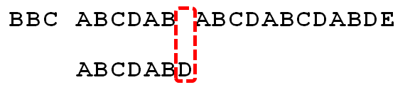
After moving 4 bits to the right, S[10] continues to match P[2]. Why move 4 bits to the right, because after moving 4 bits, there is another "AB" in the pattern string that can continue to correspond with S[8]S[9], so that I don't have to trace back. Equivalent to finding the same prefix and suffix in the pattern string substring of the character D, and then finding the next array based on the prefix suffix, and finally matching based on the next array (don't care how the next array is obtained, just want to see the matching process is For example, you can jump directly to Section 3.3.4 below.
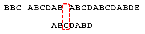
How to find a next array
From the above, we already know that the maximum common element lengths of the prefix suffixes of the string "ABCDABD" are:
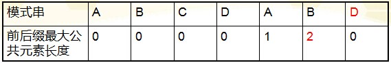
Moreover, according to this table, the following conclusions can be drawn:
When mismatched, the number of digits of the pattern string moving to the right is: number of matched characters - the maximum length value corresponding to the previous character of the mismatched character
When using this table and conclusions to match, we found that when matching a character mismatch, it is not necessary to consider the currently mismatched characters, not to mention the mismatched characters we see each time we mismatch. The maximum length value corresponding to the previous character. This leads to the next array.
Given the string "ABCDABD", you can find its next array as follows:

After comparing the next array with the maximum length table obtained before, it is not difficult to find that the next array is equivalent to the "maximum length value". The whole one is shifted to the right by one bit, and then the initial value is assigned as - 1. Realizing this, you will be surprised that the solution of the original array is so simple: it is to find the prefix suffix of the largest symmetrical length, and then shift the whole right one bit, the initial value is assigned to -1 (of course, you can also directly calculate a certain The next value corresponding to the character is the same prefix suffix of the length of the string before the character.
In other words, for a given pattern string: ABCDABD, its maximum length table and next array are as follows:
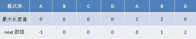
Intelligent Recommendation
Common sorting algorithms (summary)
Overview of common sorting algorithms Algorithm name time complexity Space complexity stability Bubble Sort O(N2) O(1) Unstable Select sort O(N2) O(1) Unstable Insertion sort O(N2) O(1) stable Merge s...
Summary of common encryption algorithms
Message summary Message Digest is also known as Digital Digest It is a fixed-length value that uniquely corresponds to a message or text, which is generated by a one-way Hash encryption function actin...
Summary of STL common algorithms
STL's algorithm simple concept Algorithm is a general program for use in various containers with template technology. Algorithm often operates container elements indirectly through an iterator, and ty...
Summary of common functions in algorithms
Common custom function in the algorithm Today, let's summarize some of the functions commonly used in the calculation. These functions need to be written by us, and now to summarize the following, it ...
Several common algorithms summary
In fact, the non-map graph can be seen as a special figure, so their representation methods and related algorithms are actually the same. First, BFS This is a template for Figure BFS. This is easier t...
More Recommendation
Introduction to common algorithms
First, divide and conquer The divide-and-conquer method is the law of divide and conquer. The core idea is to say that a big problem that is difficult to solve directly is divided into two or more sub...

Introduction to common algorithms in Python
First, the algorithm introduction 1. What is the algorithm? The algorithm refers to the accurate and complete description of the solution, and is a series of clear instructions to solve the problem. T...

Introduction of common hashing algorithms
background knowledge: Hash algorithms are mainly used in cache distributed systems. Distributed means that a whole is divided into multiple parts, which are executed by multiple servers. Pay attention...
Impala SQL implementation a year-on-year calculation (LAG function)
First, year-on-year In contrast to the same month data in the previous year, the "year-on-year" is called "previously" Lag (col, n, default) is used in the statistical window to th...
[Han Jiangxue] Go implements object pool mode
Object Pool Pattern Object pool mode is a creational mode, which predicts the objects to be used according to demand, creates them in advance and stores them in memory. achieve Object pool...