Preface

Sort out the optimization algorithms used before to facilitate the reproduction of Learning to learn by gradient descent by gradient descent paper work. The author uses LSTM optimizer to replace traditional optimizers such as (SGD, RMSProp, Adam, etc.), and then uses gradient descent to optimize The optimizer itself, if you are interested, you can take a look at this paper. It’s a little bit to accumulate a little. What will be the final result?

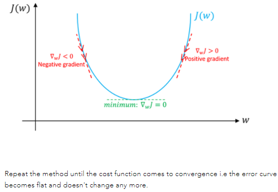
1. Gradient Descent

Gradient descentIt is an iterative method that can be used to solve least squares problems (both linear and nonlinear). When solving the model parameters of the machine learning algorithm, that is, the unconstrained optimization problem,Gradient descent(Gradient Descent) is one of the most commonly used methods
$Suppose the model g(x)=W^T x+b\\The loss function is: J(\theta) = \frac{1}{2} \sum_{i=0} ^n (g_\theta(x^{(i)})-y^{(i)})^2\\ Then the gradient update algorithm is: dW := dW-\alpha \frac{dJ(\theta)} {dW},db := db-\alpha \frac{dJ(\theta)}{db}$falseAssumemoldtypeg(x)=WTx+bdamageLoseletternumberfor：J(θ)=21​i=0∑n​(gθ​(x(i))−y(i))2thatWhatladderdegreemorenewCalculatelawfor：dW:=dW−αdWdJ(θ)​,db:=db−αdbdJ(θ)​
pyhton implementation code

def update_parameters_with_gd(parameters, grads, learning_rate):
    L = len(parameters) // 2 # Number of neural network layers

    # Update gradient
    for l in range(L):
        parameters["W" + str(l+1)] = parameters["W" + str(l + 1)] - learning_rate * grads["dW" + str(l + 1)]
        parameters["b" + str(l+1)] = parameters["b" + str(l + 1)] - learning_rate * grads["db" + str(l + 1)]
        
    return parameters

Batch Gradient Descent

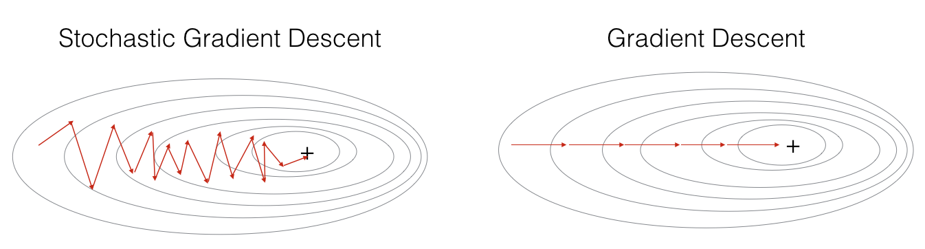
Batch gradient descentIs the most primitive form, it refers toEvery iterationuseAll samplesTo update the gradient

advantage:
   (1) One iteration is to perform calculations on all samples. At this time, the matrix is ​​used to perform operations to achieve parallelism.
  (2) The direction determined by the full data set can better represent the sample population, and thus more accurately face the direction of the extreme value. When the objective function is a convex function, BGD must be able to obtain the global optimum.
Disadvantages:
   (1) When the number of samples mm is large, all samples need to be calculated in each iteration step, and the training process will be slow. In terms of the number of iterations, the number of BGD iterations is relatively small.

Stochastic Gradient Descent

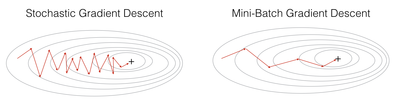
Stochastic gradient descentUnlike batch gradient descent, stochastic gradient descent isEvery iterationuseA sampleTo update the parameters. Makes training speed faster.

advantage:
   (1) Because it is not the loss function on all training data, but in each iteration, the loss function on a certain piece of training data is randomly optimized, so that each round of parameter update The speed is greatly accelerated.
Disadvantages:
  (1) The accuracy is reduced. Because even when the objective function is a strong convex function, SGD still cannot achieve linear convergence.
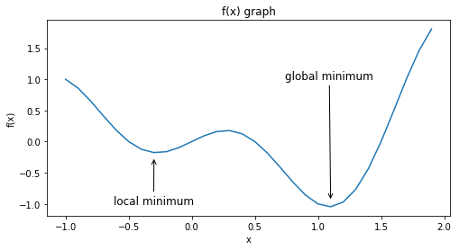
  (2) may converge to a local optimum, because a single sample cannot represent the trend of the entire sample.
  (3) is not easy to implement in parallel.

2. Exponential weighted average

Exponential weighted average(Exponentially weighted averges), also called exponentially weighted moving average, is a commonly used method of processing sequence data.
$V_i=\beta V_{i-1}+(1-\beta)\theta_t$Vi​=βVi−1​+(1−β)θt​

$V_i: is to replace the estimated value of θ_t, that is, the exponentially weighted average of the t day \\ θ_t: is the actual value of the t day Observed value \\ β: is the weight of V_{t-1}, which is an adjustable hyperparameter. (0 <β <1)$Vi​:Yeswantgenerationforθt​ofestimatemetervalue，and alsoonYesFirsttdayofMeansnumberplusrightlevelallvalueθt​:forFirsttdayofrealOccasionViewObservevalueβ：forVt−1​ofrightweight，YescanTuneSectionofultraParticipate。(0<β<1)

When using exponential weighted average, if the deviation between the first few estimates V_t and the actual θ_t is too large, the deviation correction is required, namely:
$V_t = \frac{V_t}{1-\beta^t}$Vt​=1−βtVt​​
When t is small, β is useful; when t is large, β^t approaches 0.

3. Momentum gradient descent method (momentum)

Calculate the weighted average of the gradient and use the weighted average to follow the new gradient. Generally speaking, the momentum gradient descent is faster than the standard gradient descent.

Gradient update formula：
$V_{dw} = \beta V_{dw}+(1-\beta)dw\\V_{db} = \beta V_{db}+(1-\beta)db\\w:=w-\alpha V_{dw}\\b:=b-\alpha V_{db}\\$Vdw​=βVdw​+(1−β)dwVdb​=βVdb​+(1−β)dbw:=w−αVdw​b:=b−αVdb​
Gradient Descent each step is independent of the previous gradient, and momentum can get the previous gradient.
pyhton implementation code

def initialize_velocity(parameters):  
    L = len(parameters) // 2 # Number of neural network layers
    v = {}
    
    # Initialize velocity
    for l in range(L):
        v["dW" + str(l+1)] = np.zeros_like(parameters["W" + str(l + 1)])
        v["db" + str(l+1)] = np.zeros_like(parameters["b" + str(l + 1)])
        
    return v

def update_parameters_with_momentum(parameters, grads, v, beta, learning_rate):

    L = len(parameters) // 2 # Number of neural network layers
    
    # Update the parameters of each layer
    for l in range(L):
        # Calculate velocities
        v["dW" + str(l+1)] = beta * v["dW" + str(l + 1)] + (1 - beta) * grads["dW" + str(l + 1)]
        v["db" + str(l+1)] = beta * v["db" + str(l + 1)] + (1 - beta) * grads["db" + str(l + 1)]
        # Update parameters
        parameters["W" + str(l+1)] = parameters["W" + str(l + 1)] - learning_rate * v["dW" + str(l + 1)]
        parameters["b" + str(l+1)] = parameters["b" + str(l + 1)] - learning_rate * v["db" + str(l + 1)]
        
    return parameters, v

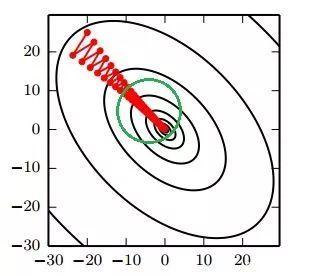
4.RMSprop（root mean square prop）

RMSPropThe full name of the algorithm is Root Mean Square Prop, which is an optimization algorithm proposed by Geoffrey E. Hinton in the Coursera course. In order to further optimize the problem of excessive swing amplitude in the update of the loss function, and further accelerate the convergence speed of the function, RMSProp The algorithm uses the gradient of weight W and bias bDifferential square weighted average。

Gradient update formula:
$S_{dw} = \beta S_{dw}+(1-\beta)d^2w\\S_{db} = \beta S_{db}+(1-\beta)d^2b\\w:=w-\alpha \frac{dw}{\sqrt{S_{dw}}}\\b:=b-\alpha \frac{db}{\sqrt{S_{db}}}\\$Sdw​=βSdw​+(1−β)d2wSdb​=βSdb​+(1−β)d2bw:=w−αSdw​ ​dw​b:=b−αSdb​ ​db​
Both RMSprop and momentum can eliminate gradient swings to a certain extent.
pyhton implementation code

def initialize_S(parameters):
   
    L = len(parameters) // 2
    s = {}
    
    for l in range(L):
        
        s["dW" + str(l+1)] = np.zeros_like(parameters["W" + str(l + 1)])
        s["db" + str(l+1)] = np.zeros_like(parameters["b" + str(l + 1)])
        
    return s

def update_parameters_with_RMSprop(parameters, grads, s, beta, learning_rate):


    L = len(parameters) 
    
    for l in range(L):
        s["dW" + str(l+1)] = beta * s["dW" + str(l + 1)] + (1 - beta) * np.square(grads["dW" + str(l + 1)])
        s["db" + str(l+1)] = beta * s["db" + str(l + 1)] + (1 - beta) * np.square(grads["db" + str(l + 1)])
        
        parameters["W" + str(l+1)] = parameters["W" + str(l + 1)] - learning_rate * grads["dW" + str(l + 1)]/np.sqrt(s["dW" + str(l + 1)]+1e-8)
        parameters["b" + str(l+1)] = parameters["b" + str(l + 1)] - learning_rate * grads["db" + str(l + 1)]/np.sqrt(s["db" + str(l + 1)]+1e-8)
        
    return parameters, s

5.Adam

With the above two optimization algorithms, one can use momentum similar to that in physics to accumulate gradients, and the other can make the convergence faster while making the amplitude of fluctuations smaller. Then the combination of the two algorithms will achieve better performance.Adam（Adaptive Moment Estimation) The algorithm is toMomentum algorithmwithRMSProp algorithmAn algorithm used in combination.

Gradient update formula:

（1）momentum
$V_{dw} = \beta_1 V_{dw}+(1-\beta_1)dw;V_{db} = \beta_1 V_{db}+(1-\beta_1)db$Vdw​=β1​Vdw​+(1−β1​)dw;Vdb​=β1​Vdb​+(1−β1​)db
（2）RMSprop
$S_{dw} = \beta_2 S_{dw}+(1-\beta_2)d^2w;S_{db} = \beta_2 S_{db}+(1-\beta_2)d^2b\\$Sdw​=β2​Sdw​+(1−β2​)d2w;Sdb​=β2​Sdb​+(1−β2​)d2b
(3) Correction deviation
$V_{dw} = \frac{V_{dw}}{1-\beta_1^t};V_{db} = \frac{V_{db}}{1-\beta_1^t}\\S_{dw} = \frac{S_{dw}}{1-\beta_1^t};S_{db} = \frac{S_{db}}{1-\beta_1^t}$Vdw​=1−β1t​Vdw​​;Vdb​=1−β1t​Vdb​​Sdw​=1−β1t​Sdw​​;Sdb​=1−β1t​Sdb​​
(4) Update
$w:=w-\alpha \frac{V_{dw}}{\sqrt{S_{dw}}};b:=b-\alpha \frac{V_{db}}{\sqrt{S_{db}}}\\$w:=w−αSdw​ ​Vdw​​;b:=b−αSdb​ ​Vdb​​
pyhton implementation code

def initialize_adam(parameters) :
  
    L = len(parameters) 
    v = {}
    s = {}
    
    for l in range(L):

        v["dW" + str(l + 1)] = np.zeros_like(parameters["W" + str(l + 1)])
        v["db" + str(l + 1)] = np.zeros_like(parameters["b" + str(l + 1)])
        
        s["dW" + str(l + 1)] = np.zeros_like(parameters["W" + str(l + 1)])
        s["db" + str(l + 1)] = np.zeros_like(parameters["b" + str(l + 1)])
    
    return v, s

def update_parameters_with_adam(parameters, grads, v, s, t, learning_rate = 0.01,
                                beta1 = 0.9, beta2 = 0.999,  epsilon = 1e-8):
    
    L = len(parameters) // 2                 
    v_corrected = {}                         
    s_corrected = {}                         
    
    
    for l in range(L):
        
        v["dW" + str(l + 1)] = beta1 * v["dW" + str(l + 1)] + (1 - beta1) * grads["dW" + str(l + 1)]
        v["db" + str(l + 1)] = beta1 * v["db" + str(l + 1)] + (1 - beta1) * grads["db" + str(l + 1)]
        
        #Calculate the estimated value after the deviation correction of the first stage, input "v, beta1, t", output: "v_corrected"
        v_corrected["dW" + str(l + 1)] = v["dW" + str(l + 1)] / (1 - np.power(beta1,t))
        v_corrected["db" + str(l + 1)] = v["db" + str(l + 1)] / (1 - np.power(beta1,t))
    
        #Calculate the moving average of the squared gradient, input: "s, grads, beta2", output: "s"
        s["dW" + str(l + 1)] = beta2 * s["dW" + str(l + 1)] + (1 - beta2) * np.square(grads["dW" + str(l + 1)])
        s["db" + str(l + 1)] = beta2 * s["db" + str(l + 1)] + (1 - beta2) * np.square(grads["db" + str(l + 1)])
         
        #Calculate the estimated value after the deviation correction of the second stage, input: "s, beta2, t", output: "s_corrected"
        s_corrected["dW" + str(l + 1)] = s["dW" + str(l + 1)] / (1 - np.power(beta2,t))
        s_corrected["db" + str(l + 1)] = s["db" + str(l + 1)] / (1 - np.power(beta2,t))
        
        #Update parameters, input: "parameters, learning_rate, v_corrected, s_corrected, epsilon". Output: "parameters".
        parameters["W" + str(l + 1)] = parameters["W" + str(l + 1)] - learning_rate * (v_corrected["dW" + str(l + 1)] / np.sqrt(s_corrected["dW" + str(l + 1)] + epsilon))
        parameters["b" + str(l + 1)] = parameters["b" + str(l + 1)] - learning_rate * (v_corrected["db" + str(l + 1)] / np.sqrt(s_corrected["db" + str(l + 1)] + epsilon))


    return parameters, v, s

---

Reference: Wu Enda Deeplearning Course