First, the algorithm introduction
1. What is the algorithm?
The algorithm refers to the accurate and complete description of the solution, and is a series of clear instructions to solve the problem. The algorithm represents a systematic way to describe the problem-solving strategy. That is to say, it is possible to obtain the required output in a limited time for a certain specification input. If an algorithm is flawed or not suitable for a problem, executing this algorithm will not solve the problem. Different algorithms may accomplish the same task with different time, space or efficiency. The pros and cons of an algorithm can be measured by space complexity and time complexity.
2, time complexity
In computer science, the time complexity of an algorithm is a function that qualitatively describes the running time of the algorithm. This is a function of the length of the string representing the input value of the algorithm. Time complexity is often expressed in large O-symbols, excluding the low-order terms and first-order coefficients of this function.
In general, the number of times the basic operations are repeatedly executed in the algorithm is a function of the problem size n, represented by T(n). If there is a helper function f(n), when n approaches infinity, T( The limit value of n)/f(n) is a constant not equal to zero, and f(n) is said to be the same magnitude function of T(n). It is denoted as T(n)=O(f(n)), and O(f(n)) is called the progressive time complexity of the algorithm (O is an order of magnitude symbol), referred to as time complexity.
Common time complexity units: efficiency goes from top to bottom,
O(1) Simple one operation (constant order)
O(n) one cycle (linear order)
O(n^2) two cycles (square order)
O(logn) cycle halved
O(nlogn) one cycle plus one cycle halved
O(n^2logn)
O(n^3)
In general, as n increases, the algorithm with the slowest growth of T(n) is the optimal algorithm.
O(1) Constant order < O(logn) Log order < O(n) Linear order < O(nlogn) < O(n^2) Square order < O(n^3) < { O(2^n) < O(n!) < O(n^n)
Big O derivation method:
- Replace all addition constants in runtime with constant 1
- In the modified run function, only the highest order item is retained
- If the highest order term exists and is not 1, remove the constant multiplied by this term
such as:
This is a piece of C code
#include "stdio.h"

int main()
{
    int i, j, x = 0, sum = 0, n = 100;    /*  Execute once */
    for( i = 1; i <= n; i++)
    {
        sum = sum + i;     /* Execute n times */
        for( j = 1; j <= n; j++)
        {
            x++;                /*  Execute n*n times */
            sum = sum + x;      /* Execute n*n this */
        }
    }
    printf("%d", sum);            /*  Execute once */
}
analysis:
Total executions = 1 + n + n*n + n*n + 1 = 2n2 + n + 2
According to the Big O derivation method:
1. Replace all addition constants in runtime with constant 1: the total number of executions is: 2n2 + n + 1
2. In the modified run times function, only the highest order term is retained, where the highest order is the quadratic of n: The total number of executions is: 2n2
3. If the highest order term exists and is not 1, remove the constant multiplied by this term, where the quadratic square of n is not 1 so the multiplication constant of this term is removed: the total number of executions is: n2
So in the end we get the algorithm time complexity of the above code is expressed as: O (n2)
3, space complexity
Space complexity is the unit used to estimate the size of the algorithm's memory footprint.
Space change time: If you need to increase the speed of the algorithm, the space required will be larger.
Second, Python implements a common sorting algorithm
The first three compare LowB, the last three compare NB
The first three time complexity are O(n^2), and the last three time complexity are O(nlog(n))
1, bubbling (exchange) sorting
Principle: Two adjacent numbers in the list. If the previous number is larger than the latter number, it is exchanged. The total number of times the list needs to be traversed is len(lst)-1
Time complexity: O(n^2)

def bubble_sort(lst):
    for i in range(len(lst) - 1):  #  This is how many times you need to loop through
        for j in range(len(lst) - 1 - i):  #  Unordered area in each array
            if lst[j] > lst[j + 1]:
                lst[j], lst[j + 1] = lst[j + 1], lst[j]


lst = [1, 2, 44, 3, 5]
bubble_sort(lst)
print(lst)
Optimization: If there is no exchange at the time of the loop, it means that the data in the sequence is already ordered.
Time complexity: The best case is 0(n), only traversing once, the general case and the worst case are O(n^2)
def bubble_sort(lst):
    for i in range(len(lst)-1):     #  This is how many times you need to loop through
        change = False      #  Make a marker variable
        for j in range(len(lst)-1-i):   #  Unordered area in each array
            if lst[j] >lst[j+1]:
                lst[j],lst[j+1] = lst[j+1],lst[j]
                change = True   #  Each time traversal, if you sort in, it will change the value of change
        if not change:  #  If the change has not changed, it means that the current sequence is ordered, just jump out of the loop.
            return


lst = [1, 2, 44, 3, 5]
bubble_sort(lst)
print(lst)
2, choose to sort
Principle: Each time the traversal finds the smallest number of the current array, and puts it in the first position, the next time you traverse the remaining unordered area, record the smallest number in the remaining list, continue to place
Time complexity O(n^2)
method one:
def select_sort(lst):
    for i in range(len(lst) - 1):  #  Current number of traversals
        min_loc = i  #  Current minimum number of positions
        for j in range(i + 1, len(lst)):  #  Disordered area
            if lst[j] < lst[min_loc]:  #  If there are smaller numbers
                lst[min_loc], lst[j] = lst[j], lst[min_loc]  #  Swap the smallest number to the current minimum number (index)


lst = [1, 2, 44, 3, 5]
select_sort(lst)
print(lst)
Method Two:
def select_sort(lst):
    for i in range(len(lst) - 1):  #  Current number of traversals
        min_loc = i  #  Current minimum number of positions
        for j in range(i + 1, len(lst)):  #  Disordered area
            if lst[j] < lst[min_loc]:  #  If there are smaller numbers
                min_loc = j  #  Minimum number of position changes
        if min_loc != i:
            lst[i], lst[min_loc] = lst[min_loc], lst[i]  #  Exchange the least number and the first number of the unordered area


lst = [1, 2, 44, 3, 5]
select_sort(lst)
print(lst)
3, insert sort
Principle: The list is divided into ordered and unordered regions. The ordered region is a relatively ordered sequence. The initial ordered region has only one element. Each time, a value is selected from the unordered region and inserted into the ordered region until there is no The sequence area is empty
Time complexity: O(n^2)
def insert_sort(lst):
    for i in range(1, len(lst)):  # Traversing from 1 means that the unordered area starts at 1, and the ordered area initially has a value.
        tmp = lst[i]  #  Tmp indicates the first card in the unordered area
        j = i - 1  #  j represents the last value of the ordered region
        while j >= 0 and lst[j] > tmp:  #  When the ordered area has a value, and the value of the ordered area is larger than the value obtained by the unordered area, it is always looped.
            lst[j + 1] = lst[j]  #  The value of the ordered area moves backward
            j -= 1  #  Find the value of the last ordered zone and then recycle
        lst[j + 1] = tmp  #  After jumping out of the loop, only the position of j+1 is empty, and the value of the current unordered area is placed at the position of j+1.


lst = [1, 2, 44, 3, 5]
insert_sort(lst)
print(lst)
4, quick sort
Idea: Take the first element, let it homing, put it in a position, make it to the left is smaller than it, the right side is bigger than it, and then recursively sort
Time complexity: O(nlog(n))
import sys
sys.setrecursionlimit(100000)  #  Set the default number of recursions


def partition(lst, left, right):
    tmp = lst[left]  #  Find a benchmark
    while left < right:
        #  Traversing from the right to the left, the number greater than the reference does not move, find the number less than the reference number assigned to the left
        while left < right and lst[right] >= tmp:
            right -= 1
        lst[left] = lst[right]  #  Find a number less than the base and assign it to the left

        #  Traverse from the left to the right, the number less than the reference does not move, find the number greater than the reference number assigned to the left
        while left < right and lst[left] <= tmp:
            left += 1
        lst[right] = lst[left]  #  Find a number greater than the baseline and assign it to the right

    lst[left] = tmp  #  Homing element
    return left  #  Return right, also the middle value


def quick_sort(lst, left, right):
    if left < right:
        mid = partition(lst, left, right)
        quick_sort(lst, left, mid-1)
        quick_sort(lst, mid+1, right)


lst = [5, 1, 6, 7, 7, 4, 2, 3, 6]
quick_sort(lst, 0, len(lst) - 1)
print(lst)
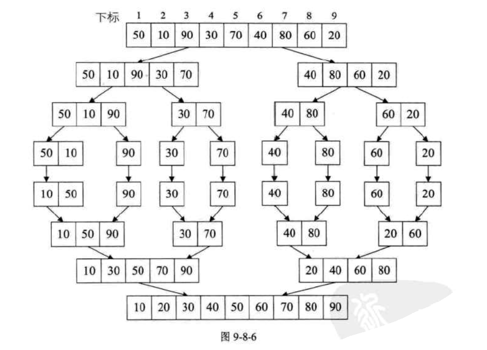
5, merge sort
Merging-ordering (MERGE-SORT) is a sorting method realized by the idea of merging. The algorithm adopts the classic divide-and-conquer strategy, which divides the problem into small problems and then recursively solves the problem. Then the "answers" of the answers obtained in the sub-stage are merged together, that is, divide and conquer.
def merge_sort(li):
    #  Recursively call itself until it is split into a single element, returning this element, no longer split
    if len(li) == 1:
        return li

    #  Take the middle position of the split
    mid = len(li) // 2
    #  After splitting, the left and right side substrings
    left = li[:mid]
    right = li[mid:]

    #  Split the left and right after splitting until there is only one element
    #  The last time recursively, ll and lr will receive a list of elements.
    #  The ll and rl before the last recursion will receive the sorted subsequence
    ll = merge_sort(left)
    rl = merge_sort(right)

    #  We sort the two split results returned and merge and return the sublist in the correct order.
    #  Here we call   a function to help us merge ll and lr in order
    return merge(ll, rl)


#  Receive two lists here
def merge(left, right):
    #  Take the data from the two ordered lists and compare them to the result.
    #  Each time we take out the smallest number of comparisons between the two lists, put the smaller one into the result
    result = []
    while len(left) > 0 and len(right) > 0:
        #  In order to maintain stability, when the encounter is equal, the number on the left is placed in the result list, because left is also the left in the large series.
        if left[0] <= right[0]:
            result.append(left.pop(0))
        else:
            result.append(right.pop(0))
    #  After the while loop comes out, indicating that one of the arrays has no data, we add another array to the result array.
    result += left
    result += right
    return result


li = [1, 5, 2, 4, 7, 5, 3, 2, 1]
li2 = merge_sort(li)
print(li2)
6, heap sorting
1. The heap is a complete binary tree
2. The complete binary tree is: if the depth of the binary tree is h, except for the hth layer, the number of nodes of the other layers (1~h-1) reaches the maximum number (2 layers), and all the nodes of the hth layer The points are continuously concentrated on the far left, which is the complete binary tree.
3. The heap satisfies two properties: Each parent of the heap has a value greater than (or less than) its child nodes, and each of the left and right subtrees of the heap is also a heap.
4. The heap is divided into a minimum heap and a maximum heap. The maximum heap is that each parent node has a larger value than the child node, and the smallest heap is that each parent node has a smaller value than the child node. To sort from small to large, we need to build the largest heap, and vice versa.
5. The heap storage is generally implemented in an array. If the array of the parent node is subscripted as i, then the subscripts of the left and right nodes are: (2*i+1) and (2*i+2). If the child node's subscript is j, then its parent node's subscript is (j-1)/2.
In a fully binary tree, if there are n elements, the last parent node in the heap is at (n/2-1).
def swap(a, b):  #  Exchange a, b
    a, b = b, a
    return a, b


def sift_down(array, start, end):
    """
         Adjusted to a large top pile, the initial pile, from bottom to top; after the top and bottom of the pile are exchanged, adjust from top to bottom
         :param array: reference to the list
         :param start: parent node
         :param end: the end of the subscript
         :return: none
    """
    while True:

        #  When the first one of the list starts with the following 0, the subscript is subscripted as i, the left child is 2*i+1, and the right child subscript is 2*i+2;
        #  If the subscript starts with 1, the left child is 2*i, and the right child is 2*i+1.
        left_child = 2 * start + 1  #  Left child's node subscript
        #  When the right child of the node exists and is greater than the left child of the node
        if left_child > end:
            break

        if left_child + 1 <= end and array[left_child + 1] > array[left_child]:
            left_child += 1
        if array[left_child] > array[start]:  #  Exchange when the maximum value of the left and right children is greater than the parent node
            array[left_child], array[start] = swap(array[left_child], array[start])

            start = left_child  #  The heap rooted at the exchange subnode after the exchange may not be a large top heap and needs to be re-adjusted
        else:  #  Exit the loop if the parent node is larger than the left and right children
            break

        print(">>", array)


def heap_sort(array):  #  Heap sort
    #  Initialize the big top heap
    first = len(array) // 2 - 1  #  The last node with children (// means rounding)
    #  The index of the first node is 0. Many blogs & textbooks start from subscript 1. It doesn't matter, you are free.
    for i in range(first, -1, -1):  #  Adjust from the last node with children
        print(array[i])
        sift_down(array, i, len(array) - 1)  #  Initialize the big top heap

    print("Initialize the big top heap result:", array)
    #  Exchange stack top and stack tail
    for head_end in range(len(array) - 1, 0, -1):  # start stop step
        array[head_end], array[0] = swap(array[head_end], array[0])  #  Exchange stack top and stack tail
        sift_down(array, 0, head_end - 1)  #  The stack length is reduced by one (head_end-1) and then adjusted from top to bottom into a large top stack.


array = [1, 1, 16, 7, 2, 3, 20, 3, 17, 8]
heap_sort(array)
print("Heap sorting end result:", array)
Third, the search algorithm
1, binary search
Binary search, also known as Binary Search, is a more efficient method of finding.However, a binary search requires that the linear table must have a sequential storage structure, and the elements in the table are ordered by keyword.。
def search(lst, num):
    left = 0
    right = len(lst) - 1
    while left <= right:  #  Cyclic condition
        mid = (left + right) // 2  #  Get the middle position, the index of the number
        if num < lst[mid]:  #  If the query number is smaller than the middle number, look for the left side of the middle number.
            right = mid - 1  #  Adjust the right border
        elif num > lst[mid]:  #  If the query number is larger than the middle number, then go to the right of the middle number to find
            left = mid + 1  #  Adjust the left border
        elif num == lst[mid]:
            print('Number found: %s, index is: %s' %(lst[mid], mid))
            return mid  #  If the query number is just an intermediate value, return the value of the index
    print('This value was not found')
    return -1  #  If the loop ends, the left side is larger than the right side, indicating that it is not found.


lst = [1, 3, 4, 8, 11, 12, 13, 15, 17, 20, 21, 27, 42, 43, 49, 51, 52, 57, 58, 59, 62, 69, 71, 73, 74, 80, 83, 84, 89, 96, 100, 111]
search(lst, 1)  #  Number found: 1, index is: 0
search(lst, 51)  #  Number found: 51, the index is: 15
search(lst, 96)  #  Number found: 96, the index is: 29
search(lst, 120)  #  This value was not found
def search(lst, num, left=None, right=None):
    left = left if left else 0
    right = len(lst)-1 if right is None else right
    mid = (right + left) // 2
    if left > right:  #  End of cycle condition
        print('This value was not found')
        return None
    elif num < lst[mid]:
        return search(lst, num, left, mid - 1)
    elif num > lst[mid]:
        return search(lst, num, mid + 1, right)
    elif lst[mid] == num:
        print('Number found: %s, index is: %s' % (lst[mid], mid))
        return mid


lst = [1, 3, 4, 8, 11, 12, 13, 15, 17, 20, 21, 27, 42, 43, 49, 51, 52, 57, 58, 59, 62, 69, 71, 73, 74, 80, 83, 84, 89, 96, 100, 111]
search(lst, 1)  #  Number found: 1, index is: 0
search(lst, 51)  #  Number found: 51, the index is: 15
search(lst, 96)  #  Number found: 96, the index is: 29
search(lst, 120)  #  This value was not found