〖Tensorflow2.0 Note 9〗: Data set loading and testing (tensor)-actual combat and supplement: about the problem of slow data set download!
| Data set loading and testing (tensor)-actual combat and supplement: about the problem of slow data set download! |
Article Directory
- 1. Data loading
- 1.1, tensorflow.keras.datasets interface
- 1.1.1, MNIST data set
- 1.1.2, cifar 10/100 data set
- 1.1.3、tf.data.Dataset.from_tensor_slices()
- 1.1.4, .shuffle() randomly shuffle
- 1.1.5, .map() data preprocessing
- 1.1.6, .batch() read a batch
- 1.2. The above methods-actual combat
- Two, test (tensor)-actual combat
- 3. Supplement: Regarding the slow downloading of data sets!
1. Data loading
- This section mainly introduces the loading of some relatively small and commonly used data sets.

1.1, tensorflow.keras.datasets interface


1.1.1, MNIST data set

- code show as below:
import tensorflow as tf
import tensorflow.keras as keras

(x,y), (x_test,y_test) = keras.datasets.mnist.load_data() #numpy format
 print(x.shape, y.shape) #y is vector
x1 = x[1,:,:]
print(y[:4])
y = tf.one_hot(y, depth=10)
print(y[:4])
print(x_test.shape,y_test.shape)
- operation result:
ssh://[email protected]:22/home/zhangkf/anaconda3/envs/tf2.0/bin/python -u /home/zhangkf/tf1/demo/TF2/cifar10.py
(60000, 28, 28) (60000,)
[5 0 4 1]
tf.Tensor(
[[0. 0. 0. 0. 0. 1. 0. 0. 0. 0.]
 [1. 0. 0. 0. 0. 0. 0. 0. 0. 0.]
 [0. 0. 0. 0. 1. 0. 0. 0. 0. 0.]
 [0. 1. 0. 0. 0. 0. 0. 0. 0. 0.]], shape=(4, 10), dtype=float32)
(10000, 28, 28) (10000,)
Process finished with exit code 0
1.1.2, cifar 10/100 data set


- The cifar10 code is as follows:
import tensorflow as tf
import tensorflow.keras as keras
import os

os.environ['TF_CPP_MIN_LOG_LEVEL'] = '2'

 (x,y), (x_test,y_test) = keras.datasets.cifar10.load_data() #numpy format
 print(x.shape, y.shape) #y is vector

print(x_test.shape,y_test.shape)
print(y[:4])
- cifar10 running results:
ssh://[email protected]:22/home/zhangkf/anaconda3/envs/tf2.0/bin/python -u /home/zhangkf/tf1/demo/TF2/cifar10.py
(50000, 32, 32, 3) (50000, 1)
(10000, 32, 32, 3) (10000, 1)
[[6]
 [9]
 [9]
 [4]]
 Process finished with exit code 0
- The cifar100 code is as follows:
import tensorflow as tf
import tensorflow.keras as keras
import os

os.environ['TF_CPP_MIN_LOG_LEVEL'] = '2'

 (x,y), (x_test,y_test) = keras.datasets.cifar100.load_data() #numpy format
 print(x.shape, y.shape) #y is vector

db = tf.data.Dataset.from_tensor_slices(x_test)
 iteration = iter(db) #1 picture
print(next(iteration).shape)

db_all = tf.data.Dataset.from_tensor_slices((x_test, y_test))
iteration_all = iter(db_all)
ob = next(iteration_all)
print(ob[0].shape)
print(ob[1].shape)
- cifar100 running results:
C:\Anaconda3\envs\tf2\python.exe E:/Codes/MyCodes/TF2/cifar100.py
(50000, 32, 32, 3) (50000, 1)
(32, 32, 3)
(32, 32, 3)
(1,)

Process finished with exit code 0
1.1.3、tf.data.Dataset.from_tensor_slices()

- code show as below:
import tensorflow as tf
import tensorflow.keras as keras
import os

os.environ['TF_CPP_MIN_LOG_LEVEL'] = '2'

 (x,y), (x_test,y_test) = keras.datasets.cifar10.load_data() #numpy format
 print(x.shape, y.shape) #y is vector

db = tf.data.Dataset.from_tensor_slices(x_test)
 iteration = iter(db) #1 picture
print(next(iteration).shape)

db_all = tf.data.Dataset.from_tensor_slices((x_test, y_test))
iteration_all = iter(db_all)
 ob = next(iteration_all) #Iterated one contains x_test, y_test
 print(ob[0].shape) #The dimension is 2, the 0th dimension is x_test
 print(ob[1].shape) #The dimension is 2, the first dimension is y_test
- operation result:
ssh://[email protected]:22/home/zhangkf/anaconda3/envs/tf2.0/bin/python -u /home/zhangkf/tf1/demo/TF2/cifar10.py
(50000, 32, 32, 3) (50000, 1)
(32, 32, 3)
(32, 32, 3)
(1,)
Process finished with exit code 0
1.1.4, .shuffle() randomly shuffle

1.1.5, .map() data preprocessing

1.1.6, .batch() read a batch


1.2. The above methods-actual combat

- The test code is as follows:
import tensorflow as tf
import tensorflow.keras as keras
import os

os.environ['TF_CPP_MIN_LOG_LEVEL'] = '2'

def prepare_mnist_features_and_labels(x,y):
    x = tf.cast(x, tf.float32) / 255.0
    y = tf.cast(y, tf.int64)
    return x,y

def mnist_dataset():
         (x,y), (x_test,y_test) = keras.datasets.fashion_mnist.load_data() #numpy in the format

         y = tf.one_hot(y, depth=10) #[10k] ==> [10k,10] tensor
    y_test = tf.one_hot(y_test, depth=10)

    ds = tf.data.Dataset.from_tensor_slices((x,y))
         ds = ds.map(prepare_mnist_features_and_labels) #Data preprocessing, note: the parameters passed in tf.map
         ds = ds.shuffle(60000).batch(100) # Randomly shuffle, read a batch sample

    ds_val = tf.data.Dataset.from_tensor_slices((x_test,y_test))
    ds_val = ds_val.map(prepare_mnist_features_and_labels)
    ds_val = ds_val.shuffle(10000).batch(100)
    return ds, ds_val


def main():
    ds, ds_val = mnist_dataset()

         print("The training set information is as follows:")
    iteration_ds = iter(ds)
    iter_ds = next(iteration_ds)
    print(iter_ds[0].shape, iter_ds[1].shape)

         print("The test set information is as follows:")
    iteration_ds_val = iter(ds_val)
    iter_ds_val = next(iteration_ds_val)
    print(iter_ds_val[0].shape, iter_ds_val[1].shape)

if __name__ == '__main__':
    main()
- The test results are as follows:
ssh://[email protected]:22/home/zhangkf/anaconda3/envs/tf2.0/bin/python -u /home/zhangkf/tf1/demo/TF2/mnist.py
 The training set information is as follows:
(100, 28, 28) (100, 10)
 The test set information is as follows:
(100, 28, 28) (100, 10)

Process finished with exit code 0
Two, test (tensor)-actual combat
- Test code
import tensorflow as tf
from tensorflow import keras
from tensorflow.keras import datasets
import os


 os.environ['TF_CPP_MIN_LOG_LEVEL']='2' #Shield irrelevant information, 2 is to print only error
 #Automatically check whether there is a mnist data set cached, if not, it will be automatically downloaded from Google.
# x: [60k, 28, 28],    x_test: [10k, 28, 28]
# y: [60k]             y_test: [10k]
(x,y),(x_test,y_test) =datasets.mnist.load_data()

 # Convert data type to tensor
#x: [0~255] => [0~ 1.]
x=tf.convert_to_tensor(x,dtype=tf.float32) / 255.
y=tf.convert_to_tensor(y,dtype=tf.int32)

x_test=tf.convert_to_tensor(x_test,dtype=tf.float32) / 255.
y_test=tf.convert_to_tensor(y_test,dtype=tf.int32)

print(x.shape, y.shape, x.dtype, y.dtype)
print(tf.reduce_min(x),tf.reduce_max(x))
print(tf.reduce_min(y),tf.reduce_max(y))


 #Create a data set, fetch one batch_size at a time, because the above fetch one at a time.
train_db = tf.data.Dataset.from_tensor_slices((x,y)).batch(128)
test_db = tf.data.Dataset.from_tensor_slices((x_test,y_test)).batch(128)

 # train_iter = iter(train_db) #iterator
# sample = next(train_iter)
# print("batch: ", sample[0].shape, sample[1].shape)

 #Create weight, complete forward propagation
#[batch,784] => [b, 256] => [b, 128] => [b, 10]
#w: [dim_in, dim_out]
#b: [dim_out]
 w1 = tf.Variable(tf.random.truncated_normal([784, 256], stddev=0.1))#The original mean value is 0, the variance dimension is 1, now the variance becomes 0.1
b1 = tf.Variable(tf.zeros([256]))
w2 = tf.Variable(tf.random.truncated_normal([256, 128], stddev=0.1))
b2 = tf.Variable(tf.zeros([128]))
w3 = tf.Variable(tf.random.truncated_normal([128, 10], stddev=0.1))
b3 = tf.Variable(tf.zeros([10]))

lr = 1e-3

 #Forward operation


 for epoch in range(100): #iterate Iterate the entire data set 10 times.
         # Outer for: Loop through all pictures.
    #for (x, y) in train_db:
         for step, (x, y) in enumerate(train_db): #Iteration for every batch
        #x: [128, 28, 28]
        #y: [128]

                 #Dimensional transformation; [b, 28, 28]-> [b, 28*28]
        x = tf.reshape(x, [-1, 28*28])
        #x: [b, 28*28]
        #h1 = x@w1 + b1
        #[b, 784]@[784, 256] + [256] = [b, 256] + [256] => [b, 256] + [b, 256]

                 #Use tensorflow to automatically derive the process, where: w,b. tf.GradientTape() The code involved in gradient calculation is put here.
        with tf.GradientTape() as tape:
                         #GradientTape only tracks the tf.Variable() type by default. If the type is not this. Here is tf.tensor, tf.Variable is a special type of tf.tensor.
                         #So simply wrap it up.

                         h1 = x@w1 + tf.broadcast_to(b1, [x.shape[0], 256]) #Direct automatic broadcast mechanism, or manually
            h1=tf.nn.relu(h1)
            #[b, 256] -> [b, 128]
            h2 = h1@w2 + b2
            h2=tf.nn.relu(h2)
            #[b, 128] -> [b, 10]
                         out = h2@w3 + b3 #Get the forward output result.

                         #computer loss: Calculate the mean square error of the error.
                         # out Dimensions: [b, 10]
                         # Real y: [b], the dimension here needs to turn y into a one-hot encoding
            y_onehot = tf.one_hot(y, depth=10)

            #mse = mean((y_onehot-out)^2)
            #shape : [b, 10]
            loss = tf.square(y_onehot - out)

            #mean: scalar
                         #loss = tf.reduce_mean(loss) / b / 10 In general, dividing by a b is enough, a mean value on each batch. It depends on how you understand it.
                         loss = tf.reduce_mean(loss) #This is equivalent to a scaling, and the positive scaling will not affect the direction of the gradient. No impact.
                         #loss = tf.sum(tf.reduce_mean(loss,axis=1)) / b, my own understanding.

                 #Get a gradient. What needs to be solved for the gradient?
        grads = tape.gradient(loss, [w1, b1, w2, b2, w3, b3])
                 #print(grads) #Result: [None, None, None, None, None, None]
                 # w1 = w1-lr* w1_grad, here for details, handwritten. Actually, you don’t need to write by hand.

                 #w1 = w1-lr * grads[0] #Here, two w1 are two objects. The original w1 subtracts this value and assigns it to a new object. W1 turns out to be
        							             #tf.Variable, after an update, the new w1 becomes tf.Tensor type. An error will occur after a new operation.
        #b1 = b1 - lr * grads[1]
        #w2 = w2 - lr * grads[2]
        #b2 = b2 - lr * grads[3]
        #w3 = w3 - lr * grads[4]
                 #b3 = b3-lr * grads[5] #First for add a step
                 w1.assign_sub(lr * grads[0]) #Update in place, the data type remains unchanged,
        b1.assign_sub(lr * grads[1])
        w2.assign_sub(lr * grads[2])
        b2.assign_sub(lr * grads[3])
        w3.assign_sub(lr * grads[4])
        b3.assign_sub(lr * grads[5])

        # print(isinstance(b3,tf.Variable))
        # print(isinstance(b3,tf.Tensor))
                 #Every 100 theory, look at the loss information.
        if step % 100 == 0:
            print(epoch, step, 'loss:', float(loss))


         # test/evluation do test
         #Note that the current (latest) must be used here [w1, b1, w2, b2, w3, b3]
    total_correct, total_number = 0, 0
    for step, (x,y) in enumerate(test_db):

        # x_test [b, 28,28] => [b, 28*28]
        x_test = tf.reshape(x, [-1, 28*28])

        # [b, 784] => [b, 256] => [b, 128] => [b, 10]
        h1 = tf.nn.relu(x_test@w1 + b1)
        h2 = tf.nn.relu(h1@w2 + b2)
        out = h2@w3 + b3

                 # out: [b, 10] Here out belongs to the range R of real numbers.
                 # prob: [b, 10] The real number range is mapped to the range [0, 1].
                 prob = tf.nn.softmax(out, axis=1) #is above the 10 dimension in [b, 10]. So axis=1
        # Predicted value: select the location with the highest probability. [b, 10] ==> [b]
        pred = tf.argmax(prob, axis=1)
        pred = tf.cast(pred, dtype=tf.int32)
                 # Real value: y: [b] Here we can find that when testing, the encoding method does not need to be converted to one-hot, only the index and pred need to be compared.
                 # [b] Int32 type.
                 # print(pred.dtype, y.dtype) Run result: <dtype:'int64'> <dtype:'int32'> Type does not match
        correct = tf.cast(tf.equal(pred, y),dtype=tf.int32)
        correct = tf.reduce_sum(correct)

                 total_correct +=int(correct) #Total correct number,
                 total_number +=x.shape[0] #Total number of tests.


         #After the loop ends:
    acc = total_correct /total_number
    print("test acc: ", acc)
- Test Results:


3. Supplement: Regarding the slow downloading of data sets!
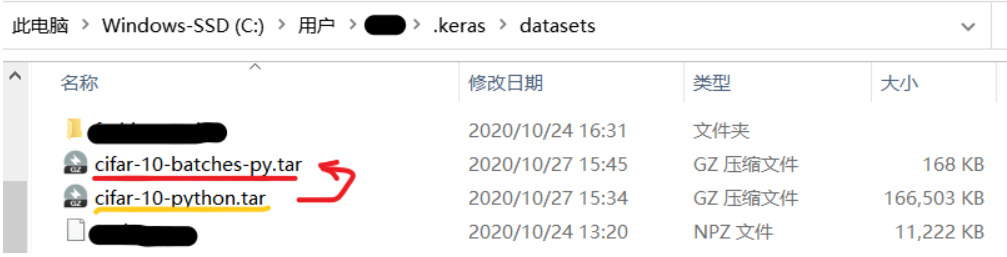
- If you can’t go over the wall to the Internet, the download speed may be very slow, and the download may be suspended automatically after a while. Here I have downloaded the data set, the file format has been sorted out, and then directly placed in the current user directory. The datasets folder in the keras directory.
- Here I have sorted out the data set on the teacher's course by myself, and can download it directly if needed:datasets data set, extraction code: jsib, The data set is shown below:

3.1, ubuntu system
- Unzip the downloaded file and put it under the following directory. If there is no datasets folder, just copy and paste it. If so, replace the following.

3.1, windows system

- If there is no datasets folder, just copy and paste it. If so, replace the following.

Intelligent Recommendation
Pytorch deep learning actual combat - loading data set
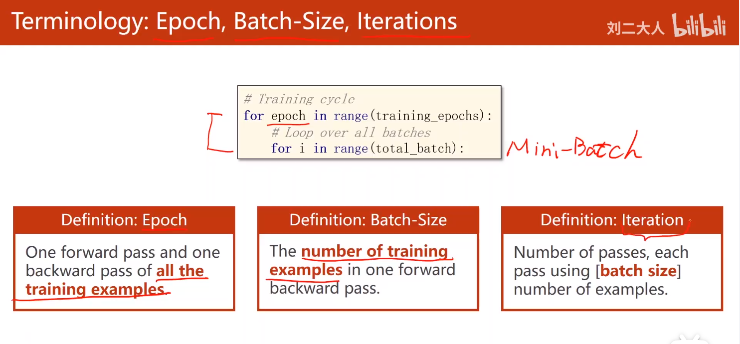
After reading Liu Er, the babysitter Pytorch tutorial, first write a note to record, interested guest officers can go to the B station. Tutorial address: First of all, distinguishBatch、Epoch with...
Integrated learning note 06 image data set actual combat
Integrated learning note 06 image data set actual combat Open source learning address:datawhale In order to consolidate the previous knowledge point, it is mainly combined with Sklearn's breast cancer...

Data mining actual combat (2) -Diam Data set (regression problem)
Articles directory 1 guide package 2 Data preparation 3 Data processing 4 model training 5 model evaluation 1 guide package 2 Data preparation 3 Data processing 4 model training Including 18 models: l...
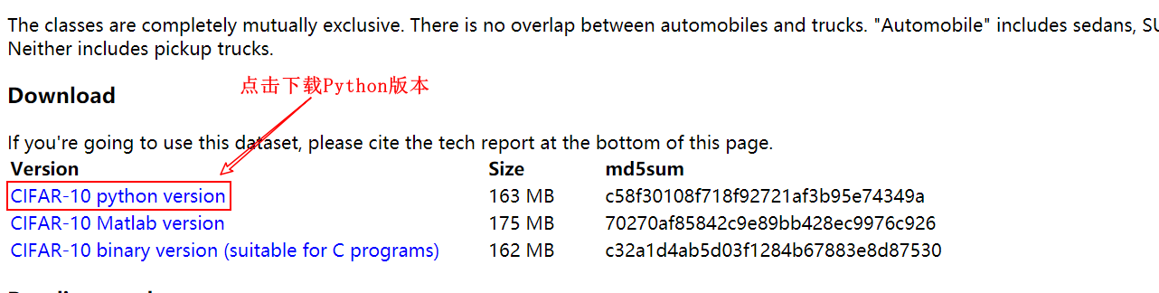
Solve the problem of slow download of cifar-10 data set in Python
Solve the slow problem of downloading the cifar-10 data set in Python Recently, I need to use the cifar-10 data set for development, but I found that the speed is very slow when using Pyth...
CIFAR-10 data set download slow problem and its solution
Disclaimer: All blog posts on this blog are records of personal learning process issues, for academic exchanges only and not for commercial use. If part of it accidentally infringes its copyright, Wan...
More Recommendation
Tensorflow2.0 data set
# Tensorflow2.0 Data Set Preparation function tf.io.read_file Read the file, return the tab of the string type, that is, the entire file is a string type tab. tf.io.decode_raw Explain a string type ta...

Tensorflow loading download data set
Tensorflow Download Data Set video https://www.bilibili.com/video/BV1jK4y187yB?p=36 image Code...

Keras download data set is slow, download data set manually
When using Keras to import the data set, we found that the download speed is very slow, then we can manually download the data set, there is a specified folder: For example, mnist dataset, when import...
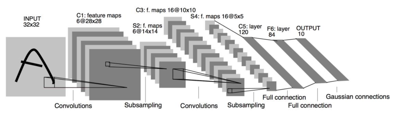
Tensorflow2.0: LeNet-5 combat identification MINIST data set
LeNet-5 model The LeNet-5 proposed in the 1990s made the convolutional neural network commercially successful at the time. The following figure is the LeNet-5 network structure diagram. It accepts 32 ...
Tensor data statistics in TensorFlow2.0
Tensors are usually large, and it is difficult to obtain useful information by directly observing the data. By obtaining the statistical information of these tensors, it is easier to infer the distrib...