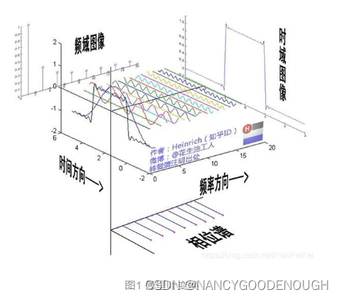
Signal analysis is for the relationship between time and frequency. The Fourier transformation provides information about the frequency domain, but the localized information about time is basically lost. Fourier transformation can only provide signalsIn the frequency of the entire time domain, the frequency information of the signal on a certain time period cannot be providedEssence Unlike Fourier's transformation,Wavelet transformationPassSmall waves(Mother Wavelet) The width of the signalFrequency domain characteristics,passDimensionSignalTime informationEssence The scaling of the mother Xiaobo is forCalculate the wavelet coefficientThese wavelet coefficients reflect the degree of correlation between wavelets and local signals. The wavelet analysis is a series of waves that decompose a signal into a series of waves that make the small waves after being shifted and shifted, soSalmonic wave is a base function of the wavelet transformationEssence The wavelet transformation can be understood as a series of small wave functions that have been shimous and shifted to replace Fourier transformation results for Fourier transformation. Compared with Fourier transformation, the wavelet transformation isLocal transformation of space (time) and frequency, Through telescopic translation, the signal is gradually carried outMulti -scale refinement, Eventually reachedHigh -frequency time subdivision，Low frequency frequency subdivision, Can automatically adapt to the requirements of the time -frequency signal analysis, so that it can focus on any detail of the signal.

• Scale function: Scaling function
• Small wave function: Wavelet function (also known as the mother function Mother Wavelet in some documents)
• The wavelet transformation is the original image and the original imageWavelet functionas well asScale functionInternal accumulation calculations, so a scale function and a small wave base function can determine a wavelet transformation

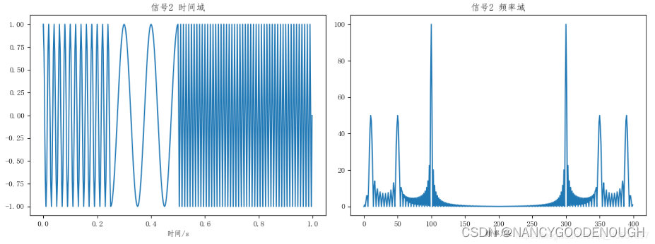
From the time of time, the two signals are very similar in frequency domain. A very natural method is to add a window (short -term distance from Fourier), divide the long -term signal into several short -term signals, and then perform Fourier transformations of each window, so as to get the frequency over time over time over time. The change, this isShort -time distance Fourier transformation

 

 Not only can you see the frequency in the signal, but you can also see when different frequency components appear.Essence Fourier transforms similar to prisms and can break down different signals. The wavelet transformation is similar to a microscope. Not only does it know what ingredients in the signal, but also where various ingredients appear.

 

 

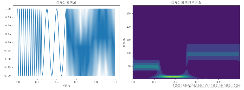
The wavelet analysis is better than Fourier's analysis::Polka analysis has good localization in time domain and frequency domainBecause the wavelet function is tightly set, and the range of sine and string is infinite interval, so the wavelet transformation can use gradually refine the time domain or airspace to replace the steps, so it canFocus on any detail of the object。

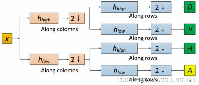
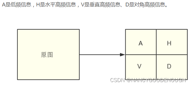
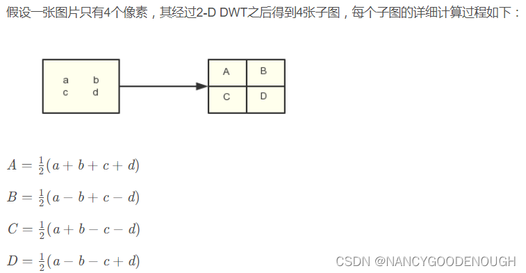
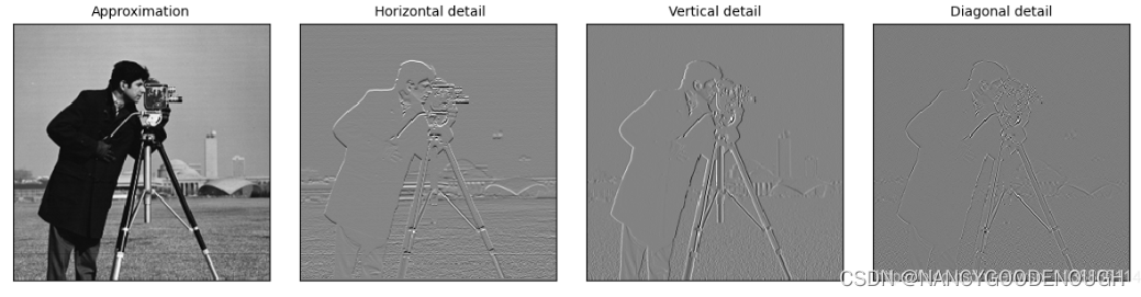
The n wave coefficient is obtained through the wavelet transformation, and the two -dimensional discrete wave transformation is input.Applying images, horizontal details, vertical details and diagonal details

 

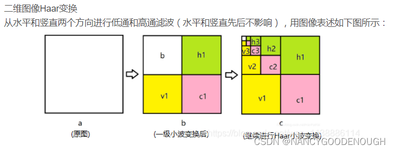
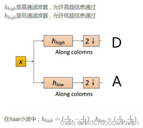
Take the HAAR wavelet transformation process as an example to understand the wavelet transformation.

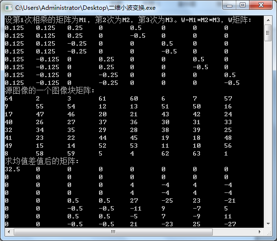
Example: Seeking the Harl wave transformation coefficient of only 4 pixels [9 7 3 5]. The calculation steps are as follows:

Step 1: Seek average, also known as APPROXIMATION. Calculate the average value of adjacent pixel pairs, get a new image with a relatively low resolution. The resolution of the new image is 1/2, and the corresponding pixel value is: [8 4]

Step 2: Differencing. Obviously, when using 2 pixels to represent this image, the image information is partially lost. In order to reconstruct the original images consisting of 4 pixels from the image of 2 pixels, the detail coeers of some images need to be stored in order to retrieve the lost information when reconstruction. The method is to use the difference between this pixel pair to divide 2, and the result is [8 4 1 -1]
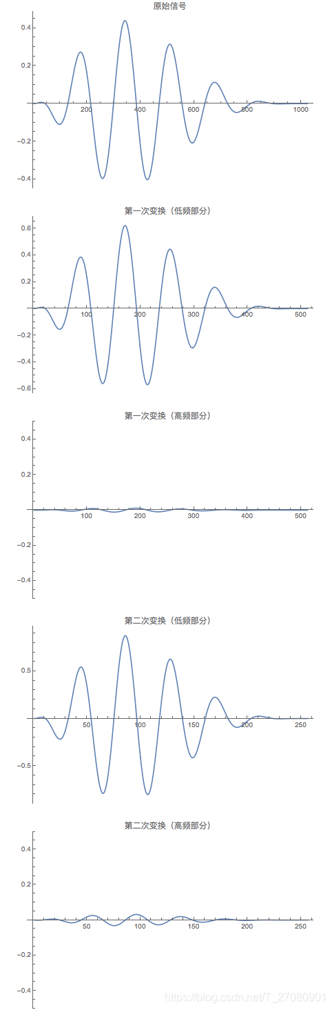
Step 3: Repeat step 1 and 2 to further decompose the image from the first step intoImage and detail coefficients with lower resolution。[6 2 1 -1]

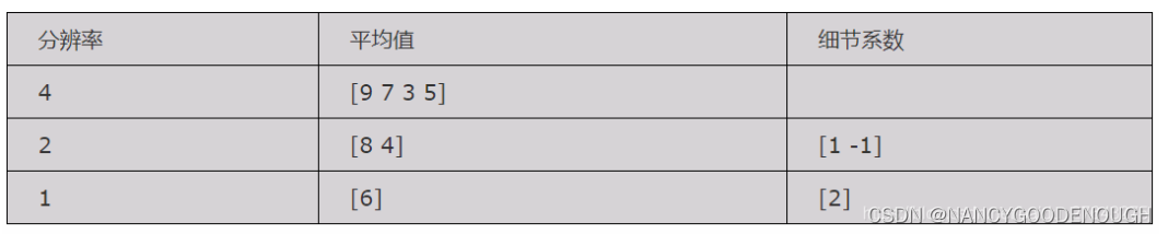
After the wavelet transformation, the image will generate low -frequency information and high -frequency information. Low -frequency information corresponds to the average value, and the high -frequency information corresponds to the difference.
The average value is a local average, the change is slow, it is low -frequency information, the contour information of the storage picture, the approximate information
The difference is the local fluctuation value, which changes faster, belongs to high -frequency information, details of the details of the storage picture, local information, and also contain noise

 

Two -dimensional discrete waves transformation

 

 

 

1. Single -level transformation of two -dimensional images:dwt2() 

haarAfter a wave of waves, after a single -level transformation:
Low -frequency informationThe range of value is: [0,510]
High -frequency informationThe range of the value is: [-255,255]

import numpy as np
import pywt
import cv2
import matplotlib.pyplot as plt

img = cv2.imread("cat.jpg")
img = cv2.resize(img, (448, 448))
 # Multi -channel image into a single channel image
img = cv2.cvtColor(img, cv2.COLOR_BGR2GRAY).astype(np.float32)

 PLT.FIGURE ('Two -dimensional waves first transformation')
coeffs = pywt.dwt2(img, 'haar')
cA, (cH, cV, cD) = coeffs

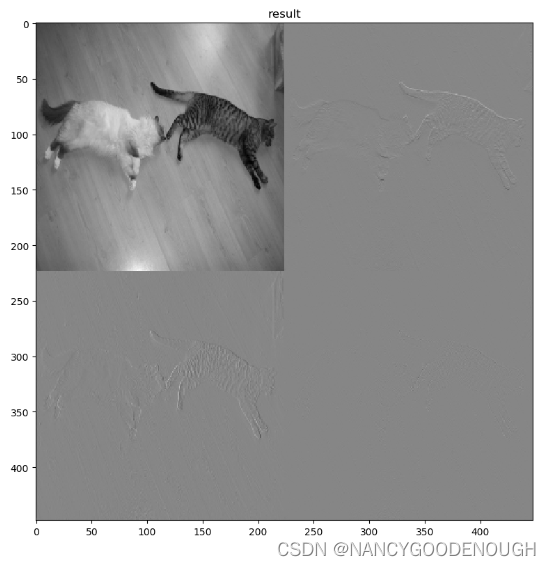
 # String each sub -diagram and finally get a picture in the end
AH = np.concatenate([cA, cH], axis=1)
VD = np.concatenate([cV, cD], axis=1)
img = np.concatenate([AH, VD], axis=0)

 # Show as gray diagram
plt.imshow(img,'gray')
plt.title('result')
plt.show()

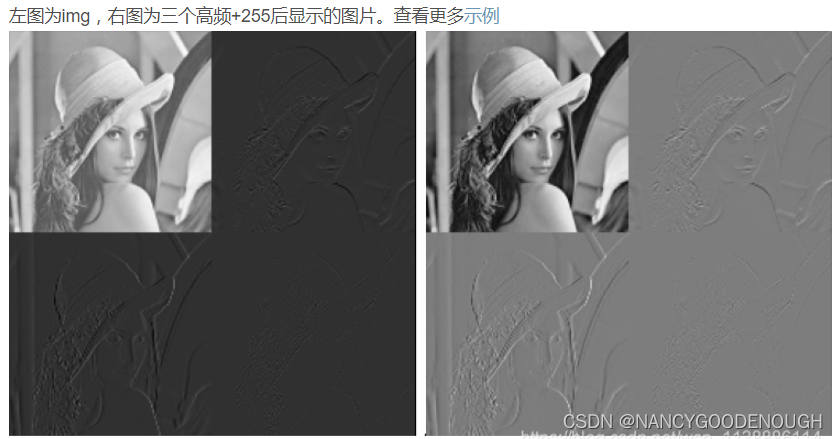
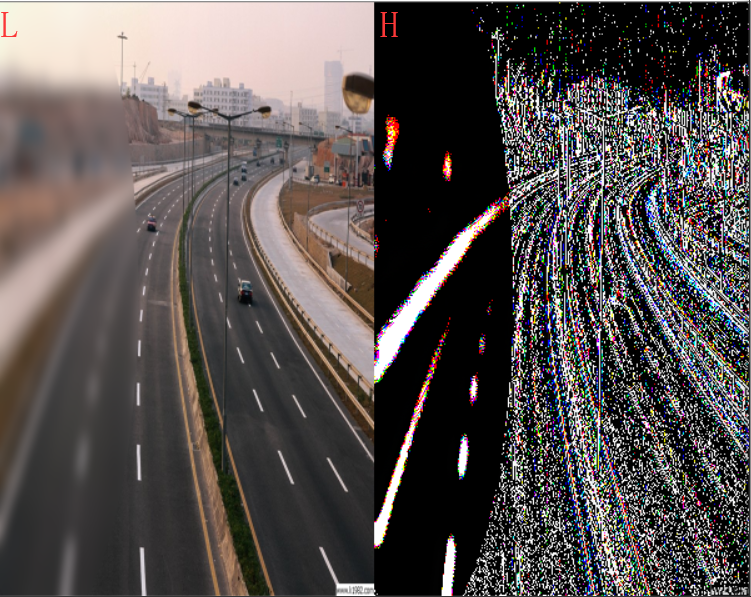
Before the stitching subgraphs, each sub -diagram should be processed. Under the circumstances, becauseThe pixel value of the high frequency part is very small or even less than 0, so the high -frequency area is black。

The easiest way to process is: add 255 high -frequency information to get the following results:

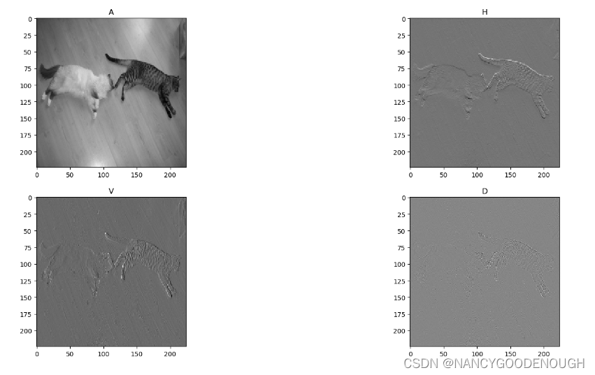
Another display method:

import numpy as np
import pywt
import cv2
import matplotlib.pyplot as plt

img = cv2.imread("cat.jpg")
img = cv2.resize(img, (448, 448))
 # Multi -channel image into a single channel image
img = cv2.cvtColor(img, cv2.COLOR_BGR2GRAY).astype(np.float32)

 PLT.FIGURE ('Two -dimensional waves first transformation')
coeffs = pywt.dwt2(img, 'haar')
cA, (cH, cV, cD) = coeffs

plt.subplot(221), plt.imshow(cA, 'gray'), plt.title("A")
plt.subplot(222), plt.imshow(cH, 'gray'), plt.title("H")
plt.subplot(223), plt.imshow(cV, 'gray'), plt.title("V")
plt.subplot(224), plt.imshow(cD, 'gray'), plt.title("D")
plt.show()

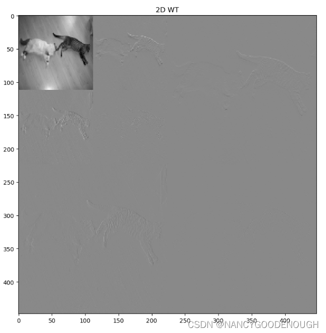
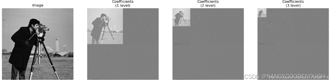
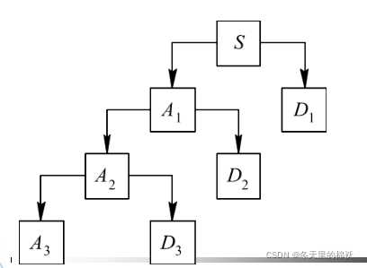
2. Multi -level decomposition of two -dimensional images:wavedec2()

import numpy as np
import pywt
import cv2
import matplotlib.pyplot as plt

img = cv2.imread("cat.jpg")
img = cv2.resize(img, (448, 448))
# img = cv2.cvtColor(img, cv2.COLOR_BGR2RGB).astype(np.float32)
img = cv2.cvtColor(img, cv2.COLOR_BGR2GRAY).astype(np.float32)

 PLT.FIGURE ('two -dimensional image multi -level decomposition')
coeffs = pywt.wavedec2(img, 'haar', level=2)
cA2, (cH2, cV2, cD2), (cH1, cV1, cD1) = coeffs

 # The pixel range of each sub -chart is naturally native to CA2 [0,255*2 ** level]
AH2 = np.concatenate([cA2, cH2+510], axis=1)
VD2 = np.concatenate([cV2+510, cD2+510], axis=1)
cA1 = np.concatenate([AH2, VD2], axis=0)

AH = np.concatenate([cA1, (cH1+255)*2], axis=1)
VD = np.concatenate([(cV1+255)*2, (cD1+255)*2], axis=1)
img = np.concatenate([AH, VD], axis=0)

plt.imshow(img,'gray')
plt.title('2D WT')
plt.show()

More examples:

 

import numpy as np
import pywt
import cv2
import matplotlib.pyplot as plt


def haar_img():
    img_u8 = cv2.imread("len_std.jpg")
    img_f32 = cv2.cvtColor(img_u8, cv2.COLOR_BGR2GRAY).astype(np.float32)

         PLT.FIGURE ('Two -dimensional waves first transformation')
    coeffs = pywt.dwt2(img_f32, 'haar')
    cA, (cH, cV, cD) = coeffs

         # String each sub -diagram and finally get a picture in the end
    AH = np.concatenate([cA, cH], axis=1)
    VD = np.concatenate([cV, cD], axis=1)
    img = np.concatenate([AH, VD], axis=0)
    return img

if __name__ == '__main__':
    img = haar_img()

    plt.imshow(img, 'gray')
    plt.title('img')
    plt.show()

DautChies (DB2) Demonstration

import numpy as np
import pywt
from matplotlib import pyplot as plt
from pywt._doc_utils import wavedec2_keys, draw_2d_wp_basis

x = pywt.data.camera().astype(np.float32)
shape = x.shape
 max_Lev = 3 # how many levels of decomposition should be drawn
 Label_levels = 3 # Figure how many layers need to be explicitly marked

fig, axes = plt.subplots(2, 4, figsize=[14, 8])
for level in range(0, max_lev + 1):
    if level == 0:
                 # Show the original image
        axes[0, 0].set_axis_off()
        axes[1, 0].imshow(x, cmap=plt.cm.gray)
        axes[1, 0].set_title('Image')
        axes[1, 0].set_axis_off()
        continue

         # Draw the border of the standard DWT base
    # draw_2d_wp_basis(shape, wavedec2_keys(level), ax=axes[0, level], label_levels=label_levels)
    # axes[0, level].set_title('{} level\ndecomposition'.format(level))

         # W d dwt
    c = pywt.wavedec2(x, 'db2', mode='periodization', level=level)

         # Independent and standardized array of each coefficient to obtain better visibility
    c[0] /= np.abs(c[0]).max()
    for detail_level in range(level):
        c[detail_level + 1] = [d / np.abs(d).max() for d in c[detail_level + 1]]

         # Show the normalization coefficient (Normalized Coefficients)
    arr, slices = pywt.coeffs_to_array(c)
    axes[1, level].imshow(arr, cmap=plt.cm.gray)
    axes[1, level].set_title('Coefficients\n({} level)'.format(level))
    axes[1, level].set_axis_off()
plt.tight_layout()
plt.show()

BIORTHOGONAL (bior) demonstration

 

import numpy as np
import matplotlib.pyplot as plt
import pywt
import pywt.data


def test_pywt():
    original = pywt.data.camera()

    # The wavelet transformation of the image, the approximation and details of the graphic
    titles = ['Approximation', ' Horizontal detail', 'Vertical detail', 'Diagonal detail']
    coeffs2 = pywt.dwt2(original, 'bior1.3')
    LL, (LH, HL, HH) = coeffs2
    plt.imshow(original)
    plt.colorbar(shrink=0.8)
    fig = plt.figure(figsize=(12, 3))
    for i, a in enumerate([LL, LH, HL, HH]):
        ax = fig.add_subplot(1, 4, i + 1)
        ax.imshow(a, interpolation="nearest", cmap=plt.cm.gray)
        ax.set_title(titles[i], fontsize=10)
        ax.set_xticks([])
        ax.set_yticks([])

    fig.tight_layout()
    plt.show()


if __name__ == '__main__':
    test_pywt()

 

 Python discrete wavelet transformation (DWT) pywt library_songpingwang's blog

 [Polaris transformation] Salmonic transformation entry ---- haar waves_1273545169 blog-CSDN blog_haar waves

 [Polar transformation] Python transformation Python implementation-Pywavelets_1273545169 blog